Lecture 8 - Law of Large Numbers and Central Limit Theorem
In the previous lectures we introduced random variables, their distributions, moments, and the joint characterization of pairs of random variables.
A natural next step is to consider a sequence of observations
ξ 1 , ξ 2 , … , ξ n , … \xi_1,\xi_2,\ldots,\xi_n,\ldots ξ 1 , ξ 2 , … , ξ n , … and to study quantities such as their sum
S n = ∑ k = 1 n ξ k S_n=\sum_{k=1}^n \xi_k S n = k = 1 ∑ n ξ k and their average
ξ ‾ n = 1 n ∑ k = 1 n ξ k = S n n . \overline{\xi}_n
=
\frac{1}{n}\sum_{k=1}^n\xi_k
=
\frac{S_n}{n}. ξ n = n 1 k = 1 ∑ n ξ k = n S n . These quantities arise naturally whenever an experiment is repeated.
For example:
a physical measurement is repeated several times;
a coin is tossed many times;
a component is tested repeatedly;
a numerical experiment is performed with random inputs;
a sample is collected from a population.
Suppose that the random variables ξ 1 , … , ξ n \xi_1,\ldots,\xi_n ξ 1 , … , ξ n
E [ ξ k ] = μ , Var ( ξ k ) = σ 2 . \mathbb{E}[\xi_k]=\mu,
\qquad
\operatorname{Var}(\xi_k)=\sigma^2. E [ ξ k ] = μ , Var ( ξ k ) = σ 2 . From the linearity of expectation,
E [ ξ ‾ n ] = μ . \mathbb{E}[\overline{\xi}_n]
=
\mu. E [ ξ n ] = μ . If the variables are independent, then
Var ( ξ ‾ n ) = σ 2 n . \operatorname{Var}(\overline{\xi}_n)
=
\frac{\sigma^2}{n}. Var ( ξ n ) = n σ 2 . Consequently,
SD ( ξ ‾ n ) = σ n . \operatorname{SD}(\overline{\xi}_n)
=
\frac{\sigma}{\sqrt{n}}. SD ( ξ n ) = n σ . The average therefore becomes increasingly concentrated around μ \mu μ n n n
This observation leads to two fundamental questions:
Does ξ ‾ n \overline{\xi}_n ξ n μ \mu μ n → ∞ n\to\infty n → ∞
If it does, how large are the fluctuations of ξ ‾ n \overline{\xi}_n ξ n μ \mu μ
The first question is answered by the Law of Large Numbers .
The second is answered by the Central Limit Theorem .
Convergence in Probability ¶ To formulate the Law of Large Numbers, we first need a notion of convergence for random variables.
Let ξ 1 , ξ 2 , … \xi_1,\xi_2,\ldots ξ 1 , ξ 2 , … ξ \xi ξ ξ n \xi_n ξ n converges in probability to ξ \xi ξ ε > 0 \varepsilon>0 ε > 0
lim n → ∞ P ( { ∣ ξ n − ξ ∣ > ε } ) = 0. \lim_{n\to\infty}
\mathbb{P}
\left(
\left\{
|\xi_n-\xi|>\varepsilon
\right\}
\right)
=
0. n → ∞ lim P ( { ∣ ξ n − ξ ∣ > ε } ) = 0. We write
ξ n → P ξ . \xi_n\xrightarrow{\mathbb{P}}\xi. ξ n P ξ . The interpretation is that, for every fixed tolerance ε > 0 \varepsilon>0 ε > 0 ξ n \xi_n ξ n ξ \xi ξ ε \varepsilon ε
Convergence in probability does not require that ξ n \xi_n ξ n ξ \xi ξ n n n
For example, if
Var ( ξ n ) ⟶ 0 \operatorname{Var}(\xi_n)\longrightarrow 0 Var ( ξ n ) ⟶ 0 and
E [ ξ n ] ⟶ μ , \mathbb{E}[\xi_n]\longrightarrow \mu, E [ ξ n ] ⟶ μ , then one expects ξ n \xi_n ξ n μ \mu μ
A Useful Consequence of Chebyshev’s Inequality ¶ Recall Chebyshev’s inequality from Lecture 6:
P ( { ∣ ξ − E [ ξ ] ∣ ≥ ε } ) ≤ Var ( ξ ) ε 2 . \mathbb{P}
\left(
\left\{
|\xi-\mathbb{E}[\xi]|\geq\varepsilon
\right\}
\right)
\leq
\frac{\operatorname{Var}(\xi)}{\varepsilon^2}. P ( { ∣ ξ − E [ ξ ] ∣ ≥ ε } ) ≤ ε 2 Var ( ξ ) . Suppose that
E [ ξ n ] = μ \mathbb{E}[\xi_n]=\mu E [ ξ n ] = μ for every n n n
Var ( ξ n ) ⟶ 0. \operatorname{Var}(\xi_n)\longrightarrow 0. Var ( ξ n ) ⟶ 0. Then
P ( ∣ ξ n − μ ∣ ≥ ε ) ≤ Var ( ξ n ) ε 2 ⟶ 0. \mathbb{P}
\left(
|\xi_n-\mu|\geq\varepsilon
\right)
\leq
\frac{\operatorname{Var}(\xi_n)}{\varepsilon^2}
\longrightarrow 0. P ( ∣ ξ n − μ ∣ ≥ ε ) ≤ ε 2 Var ( ξ n ) ⟶ 0. Therefore,
ξ n → P μ . \xi_n\xrightarrow{\mathbb{P}}\mu. ξ n P μ . This simple argument is the main tool behind the elementary form of the Law of Large Numbers.
The Weak Law of Large Numbers ¶ We can now state the fundamental result.
Let ξ 1 , ξ 2 , … \xi_1,\xi_2,\ldots ξ 1 , ξ 2 , …
E [ ξ 1 ] = μ , Var ( ξ 1 ) = σ 2 < ∞ . \mathbb{E}[\xi_1]=\mu,
\qquad
\operatorname{Var}(\xi_1)=\sigma^2<\infty. E [ ξ 1 ] = μ , Var ( ξ 1 ) = σ 2 < ∞. Then
ξ ‾ n = 1 n ∑ k = 1 n ξ k → P μ . \overline{\xi}_n
=
\frac{1}{n}\sum_{k=1}^n\xi_k
\xrightarrow{\mathbb{P}}
\mu. ξ n = n 1 k = 1 ∑ n ξ k P μ . By linearity of expectation,
E [ ξ ‾ n ] = μ . \mathbb{E}[\overline{\xi}_n]=\mu. E [ ξ n ] = μ . Since the random variables are independent,
Var ( ξ ‾ n ) = σ 2 n . \operatorname{Var}(\overline{\xi}_n)
=
\frac{\sigma^2}{n}. Var ( ξ n ) = n σ 2 . Chebyshev’s inequality therefore gives, for every ε > 0 \varepsilon>0 ε > 0
P ( ∣ ξ ‾ n − μ ∣ ≥ ε ) ≤ σ 2 n ε 2 . \mathbb{P}
\left(
|\overline{\xi}_n-\mu|\geq\varepsilon
\right)
\leq
\frac{\sigma^2}{n\varepsilon^2}. P ( ∣ ξ n − μ ∣ ≥ ε ) ≤ n ε 2 σ 2 . The right-hand side tends to zero as n → ∞ n\to\infty n → ∞
ξ ‾ n → P μ . \overline{\xi}_n\xrightarrow{\mathbb{P}}\mu. ξ n P μ . The theorem says that the average of a large number of independent observations approaches the common expected value.
This provides a mathematical foundation for the idea that repeated measurements can reveal an underlying mean.
Suppose that a physical quantity has true value a a a
ξ k = a + ε k , \xi_k=a+\varepsilon_k, ξ k = a + ε k , where the errors ε k \varepsilon_k ε k
E [ ε k ] = 0 , Var ( ε k ) = σ 2 . \mathbb{E}[\varepsilon_k]=0,
\qquad
\operatorname{Var}(\varepsilon_k)=\sigma^2. E [ ε k ] = 0 , Var ( ε k ) = σ 2 . Then
E [ ξ k ] = a . \mathbb{E}[\xi_k]=a. E [ ξ k ] = a . The average measurement is
ξ ‾ n = a + 1 n ∑ k = 1 n ε k . \overline{\xi}_n
=
a+
\frac{1}{n}\sum_{k=1}^n\varepsilon_k. ξ n = a + n 1 k = 1 ∑ n ε k . The Weak Law of Large Numbers gives
ξ ‾ n → P a . \overline{\xi}_n\xrightarrow{\mathbb{P}}a. ξ n P a . Thus, averaging independent measurements removes the random error in the limit.
The variance of the averaged error is
Var ( ξ ‾ n − a ) = σ 2 n . \operatorname{Var}(\overline{\xi}_n-a)
=
\frac{\sigma^2}{n}. Var ( ξ n − a ) = n σ 2 . This explains quantitatively why averaging repeated measurements improves precision.
The Law of Large Numbers for Bernoulli Trials ¶ Consider independent Bernoulli random variables
ξ k = { 1 , success , 0 , failure , \xi_k=
\begin{cases}
1,&\text{success},\\
0,&\text{failure},
\end{cases} ξ k = { 1 , 0 , success , failure , with
P ( { ξ k = 1 } ) = p . \mathbb{P}(\{\xi_k=1\})=p. P ({ ξ k = 1 }) = p . The sum
S n = ∑ k = 1 n ξ k S_n=\sum_{k=1}^n\xi_k S n = k = 1 ∑ n ξ k counts the number of successes in n n n
The fraction of successes is
S n n = ξ ‾ n . \frac{S_n}{n}
=
\overline{\xi}_n. n S n = ξ n . Since
E [ ξ k ] = p , \mathbb{E}[\xi_k]=p, E [ ξ k ] = p , the Weak Law of Large Numbers gives
S n n → P p . \frac{S_n}{n}
\xrightarrow{\mathbb{P}}
p. n S n P p . Thus, for a large number of independent trials, the observed relative frequency of success is close to the probability of success.
This provides a rigorous connection between probability and relative frequency.
Suppose that each manufactured component has probability p = 0.02 p=0.02 p = 0.02
Let ξ k \xi_k ξ k k k k
1 n ∑ k = 1 n ξ k \frac{1}{n}\sum_{k=1}^n\xi_k n 1 k = 1 ∑ n ξ k is the observed defect rate among the first n n n
The Law of Large Numbers gives
1 n ∑ k = 1 n ξ k → P 0.02. \frac{1}{n}\sum_{k=1}^n\xi_k
\xrightarrow{\mathbb{P}}
0.02. n 1 k = 1 ∑ n ξ k P 0.02. Hence, as the number of inspected components becomes large, the observed defect rate becomes close to 2 % 2\% 2%
Strong Law of Large Numbers ¶ There is a stronger form of the Law of Large Numbers.
The distinction concerns the mode of convergence.
The Weak Law gives convergence in probability:
ξ ‾ n → P μ . \overline{\xi}_n\xrightarrow{\mathbb{P}}\mu. ξ n P μ . The Strong Law gives almost sure convergence :
P ( { lim n → ∞ ξ ‾ n = μ } ) = 1. \mathbb{P}
\left(
\left\{
\lim_{n\to\infty}\overline{\xi}_n=\mu
\right\}
\right)
=
1. P ( { n → ∞ lim ξ n = μ } ) = 1. We write
ξ ‾ n → a.s. μ . \overline{\xi}_n\xrightarrow{\text{a.s.}}\mu. ξ n a.s. μ . Let ξ 1 , ξ 2 , … \xi_1,\xi_2,\ldots ξ 1 , ξ 2 , …
E [ ∣ ξ 1 ∣ ] < ∞ . \mathbb{E}[|\xi_1|]<\infty. E [ ∣ ξ 1 ∣ ] < ∞. Then
ξ ‾ n → a.s. E [ ξ 1 ] . \overline{\xi}_n
\xrightarrow{\text{a.s.}}
\mathbb{E}[\xi_1]. ξ n a.s. E [ ξ 1 ] . The Strong Law is a deeper result than the Weak Law. Its proof requires tools beyond those developed in this course, so we will use the result without proving it.
Almost sure convergence is stronger than convergence in probability. In particular,
ξ n → a.s. ξ ⟹ ξ n → P ξ . \xi_n\xrightarrow{\text{a.s.}}\xi
\quad\Longrightarrow\quad
\xi_n\xrightarrow{\mathbb{P}}\xi. ξ n a.s. ξ ⟹ ξ n P ξ . The converse is not true in general.
For practical applications, both versions express the same fundamental principle: sufficiently many independent observations reveal the underlying mean.
Why the Law of Large Numbers Is Not the Whole Story ¶ The Law of Large Numbers tells us that
ξ ‾ n ≈ μ \overline{\xi}_n\approx\mu ξ n ≈ μ for large n n n
But it does not tell us how the random error
ξ ‾ n − μ \overline{\xi}_n-\mu ξ n − μ behaves.
From Lecture 6,
SD ( ξ ‾ n ) = σ n . \operatorname{SD}(\overline{\xi}_n)
=
\frac{\sigma}{\sqrt{n}}. SD ( ξ n ) = n σ . This suggests that the natural scale of the fluctuations is
1 n . \frac{1}{\sqrt{n}}. n 1 . Therefore, instead of studying ξ ‾ n − μ \overline{\xi}_n-\mu ξ n − μ
Z n = ξ ‾ n − μ σ / n = n ( ξ ‾ n − μ ) σ . Z_n
=
\frac{\overline{\xi}_n-\mu}{\sigma/\sqrt{n}}
=
\frac{\sqrt{n}(\overline{\xi}_n-\mu)}{\sigma}. Z n = σ / n ξ n − μ = σ n ( ξ n − μ ) . Using S n = n ξ ‾ n S_n=n\overline{\xi}_n S n = n ξ n
Z n = S n − n μ σ n . Z_n
=
\frac{S_n-n\mu}{\sigma\sqrt{n}}. Z n = σ n S n − n μ . The Central Limit Theorem describes the limiting distribution of Z n Z_n Z n
Convergence in Distribution ¶ Before stating the theorem, we introduce another form of convergence.
Let F n F_n F n ξ n \xi_n ξ n F F F ξ \xi ξ
We say that ξ n \xi_n ξ n converges in distribution to ξ \xi ξ
lim n → ∞ F n ( x ) = F ( x ) \lim_{n\to\infty}F_n(x)=F(x) n → ∞ lim F n ( x ) = F ( x ) at every point x x x F F F
We write
ξ n → d ξ . \xi_n\xrightarrow{d}\xi. ξ n d ξ . Convergence in distribution concerns the limiting shape of the probability distributions. It does not necessarily mean that the random variables themselves become close for individual outcomes.
For the Central Limit Theorem, the limiting random variable is a standard normal random variable. Thus the theorem is a statement about the convergence of distribution functions, not about the original observations becoming normally distributed.
The Central Limit Theorem ¶ We can now state one of the central results of probability theory.
Let ξ 1 , ξ 2 , … \xi_1,\xi_2,\ldots ξ 1 , ξ 2 , …
E [ ξ 1 ] = μ \mathbb{E}[\xi_1]=\mu E [ ξ 1 ] = μ and
0 < Var ( ξ 1 ) = σ 2 < ∞ . 0<\operatorname{Var}(\xi_1)=\sigma^2<\infty. 0 < Var ( ξ 1 ) = σ 2 < ∞. Then
S n − n μ σ n → d Z , Z ∼ N ( 0 , 1 ) . \frac{S_n-n\mu}{\sigma\sqrt{n}}
\xrightarrow{d}
Z,
\qquad
Z\sim N(0,1). σ n S n − n μ d Z , Z ∼ N ( 0 , 1 ) . Equivalently,
n ( ξ ‾ n − μ ) σ → d N ( 0 , 1 ) . \frac{\sqrt{n}(\overline{\xi}_n-\mu)}
{\sigma}
\xrightarrow{d}
N(0,1). σ n ( ξ n − μ ) d N ( 0 , 1 ) . The theorem says that, after centering by the mean and scaling by the standard deviation, the distribution of the sum approaches a standard normal distribution.
Equivalently, for large n n n
ξ ‾ n ≈ N ( μ , σ 2 n ) . \overline{\xi}_n
\approx
N\left(
\mu,\frac{\sigma^2}{n}
\right). ξ n ≈ N ( μ , n σ 2 ) . This approximation is one of the main reasons why the normal distribution appears throughout statistics, experimental science, engineering, and numerical analysis.
Interpreting the Central Limit Theorem ¶ The Law of Large Numbers and the Central Limit Theorem answer different questions.
The Law of Large Numbers says
ξ ‾ n ⟶ μ , \overline{\xi}_n\longrightarrow\mu, ξ n ⟶ μ , in an appropriate sense.
The Central Limit Theorem says that the fluctuations around μ \mu μ 1 / n 1/\sqrt{n} 1/ n
ξ ‾ n − μ ≈ σ n Z , Z ∼ N ( 0 , 1 ) . \overline{\xi}_n-\mu
\approx
\frac{\sigma}{\sqrt{n}}Z,
\qquad
Z\sim N(0,1). ξ n − μ ≈ n σ Z , Z ∼ N ( 0 , 1 ) . Thus, for large n n n
ξ ‾ n ≈ μ + σ n Z . \overline{\xi}_n
\approx
\mu+\frac{\sigma}{\sqrt{n}}Z. ξ n ≈ μ + n σ Z . This formula contains both the Law of Large Numbers and the Central Limit Theorem:
the factor 1 / n 1/\sqrt{n} 1/ n μ \mu μ
the random fluctuation is approximately Gaussian.
The two theorems therefore describe different aspects of the same asymptotic phenomenon.
Approximate Probabilities for Sample Averages ¶ The Central Limit Theorem can be used to approximate probabilities involving ξ ‾ n \overline{\xi}_n ξ n
Suppose that a < b a<b a < b n n n
P ( a ≤ ξ ‾ n ≤ b ) ≈ P ( a − μ σ / n ≤ Z ≤ b − μ σ / n ) , \mathbb{P}(a\leq\overline{\xi}_n\leq b)
\approx
\mathbb{P}
\left(
\frac{a-\mu}{\sigma/\sqrt{n}}
\leq
Z
\leq
\frac{b-\mu}{\sigma/\sqrt{n}}
\right), P ( a ≤ ξ n ≤ b ) ≈ P ( σ / n a − μ ≤ Z ≤ σ / n b − μ ) , where Z ∼ N ( 0 , 1 ) Z\sim N(0,1) Z ∼ N ( 0 , 1 )
If Φ \Phi Φ
P ( a ≤ ξ ‾ n ≤ b ) ≈ Φ ( ( b − μ ) n σ ) − Φ ( ( a − μ ) n σ ) . \mathbb{P}(a\leq\overline{\xi}_n\leq b)
\approx
\Phi
\left(
\frac{(b-\mu)\sqrt{n}}{\sigma}
\right)
-
\Phi
\left(
\frac{(a-\mu)\sqrt{n}}{\sigma}
\right). P ( a ≤ ξ n ≤ b ) ≈ Φ ( σ ( b − μ ) n ) − Φ ( σ ( a − μ ) n ) . This gives a practical way to compute probabilities involving averages even when the original distribution of ξ k \xi_k ξ k
Suppose that independent measurements satisfy
E [ ξ k ] = a , SD ( ξ k ) = σ . \mathbb{E}[\xi_k]=a,
\qquad
\operatorname{SD}(\xi_k)=\sigma. E [ ξ k ] = a , SD ( ξ k ) = σ . Suppose that n = 100 n=100 n = 100
Then
SD ( ξ ‾ 100 ) = σ 10 . \operatorname{SD}(\overline{\xi}_{100})
=
\frac{\sigma}{10}. SD ( ξ 100 ) = 10 σ . By the Central Limit Theorem,
ξ ‾ 100 ≈ N ( a , σ 2 100 ) . \overline{\xi}_{100}
\approx
N\left(a,\frac{\sigma^2}{100}\right). ξ 100 ≈ N ( a , 100 σ 2 ) . Consequently,
P ( ∣ ξ ‾ 100 − a ∣ ≤ σ 10 ) ≈ P ( ∣ Z ∣ ≤ 1 ) . \mathbb{P}
\left(
|\overline{\xi}_{100}-a|
\leq
\frac{\sigma}{10}
\right)
\approx
\mathbb{P}(|Z|\leq1). P ( ∣ ξ 100 − a ∣ ≤ 10 σ ) ≈ P ( ∣ Z ∣ ≤ 1 ) . For a standard normal random variable,
P ( ∣ Z ∣ ≤ 1 ) = 2 Φ ( 1 ) − 1 ≈ 0.6827. \mathbb{P}(|Z|\leq1)
=
2\Phi(1)-1
\approx
0.6827. P ( ∣ Z ∣ ≤ 1 ) = 2Φ ( 1 ) − 1 ≈ 0.6827. Thus, approximately 68.27 % 68.27\% 68.27%
The De Moivre--Laplace Theorem ¶ The normal approximation to the binomial distribution introduced in Lecture 5 is a special case of the Central Limit Theorem.
Let
ξ 1 , … , ξ n \xi_1,\ldots,\xi_n ξ 1 , … , ξ n be independent Bernoulli random variables with parameter p p p
Then
E [ ξ k ] = p , Var ( ξ k ) = p ( 1 − p ) . \mathbb{E}[\xi_k]=p,
\qquad
\operatorname{Var}(\xi_k)=p(1-p). E [ ξ k ] = p , Var ( ξ k ) = p ( 1 − p ) . The sum
S n = ∑ k = 1 n ξ k S_n=\sum_{k=1}^n\xi_k S n = k = 1 ∑ n ξ k has a binomial distribution:
S n ∼ Bin ( n , p ) . S_n\sim\operatorname{Bin}(n,p). S n ∼ Bin ( n , p ) . Applying the Central Limit Theorem gives
S n − n p n p ( 1 − p ) → d N ( 0 , 1 ) . \frac{S_n-np}
{\sqrt{np(1-p)}}
\xrightarrow{d}
N(0,1). n p ( 1 − p ) S n − n p d N ( 0 , 1 ) . This is the De Moivre--Laplace theorem .
For large n n n
S n ≈ N ( n p , n p ( 1 − p ) ) . S_n
\approx
N\left(np,np(1-p)\right). S n ≈ N ( n p , n p ( 1 − p ) ) . This explains the normal approximation to the binomial distribution discussed previously.
Continuity correction ¶ The binomial random variable is discrete, whereas the normal distribution is continuous.
When approximating a binomial probability using a normal distribution, a continuity correction can improve the approximation.
For example,
P ( S n ≤ k ) ≈ Φ ( k + 1 2 − n p n p ( 1 − p ) ) . \mathbb{P}(S_n\leq k)
\approx
\Phi
\left(
\frac{k+\frac12-np}
{\sqrt{np(1-p)}}
\right). P ( S n ≤ k ) ≈ Φ ( n p ( 1 − p ) k + 2 1 − n p ) . Similarly,
P ( S n = k ) ≈ Φ ( k + 1 2 − n p n p ( 1 − p ) ) − Φ ( k − 1 2 − n p n p ( 1 − p ) ) . \mathbb{P}(S_n=k)
\approx
\Phi
\left(
\frac{k+\frac12-np}
{\sqrt{np(1-p)}}
\right)
-
\Phi
\left(
\frac{k-\frac12-np}
{\sqrt{np(1-p)}}
\right). P ( S n = k ) ≈ Φ ( n p ( 1 − p ) k + 2 1 − n p ) − Φ ( n p ( 1 − p ) k − 2 1 − n p ) . The correction accounts for the fact that the integer value k k k k − 1 2 k-\frac12 k − 2 1 k + 1 2 k+\frac12 k + 2 1
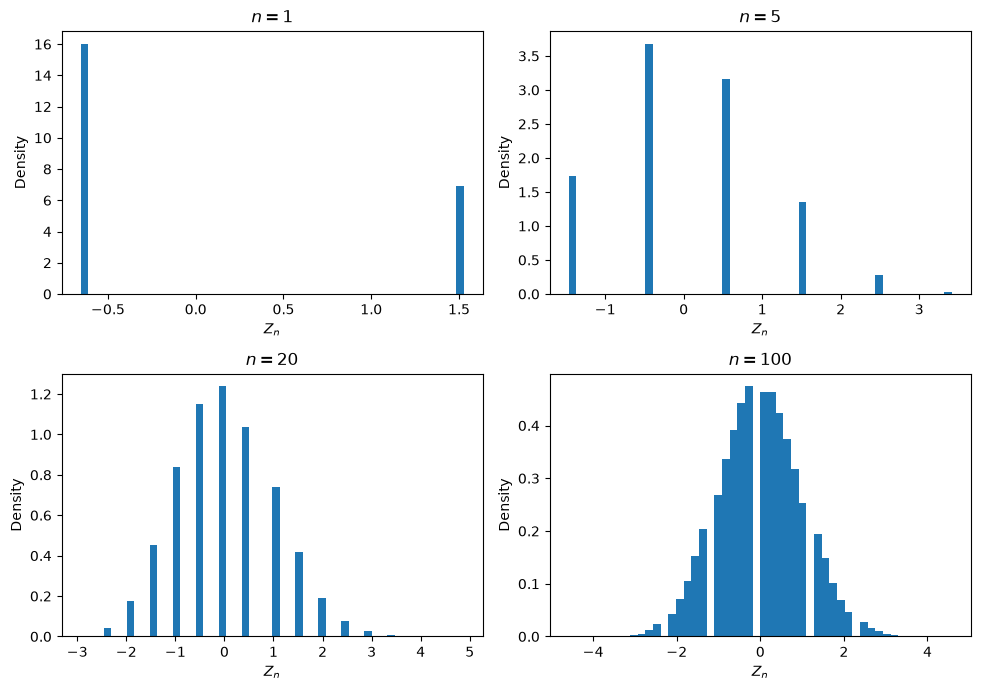
Numerical Illustration of the Central Limit Theorem ¶ The Central Limit Theorem is remarkable because the original distribution can be very different from the normal distribution.
For example, consider a Bernoulli random variable with
For each n n n
ξ 1 , … , ξ n \xi_1,\ldots,\xi_n ξ 1 , … , ξ n and compute
Z n = n ( ξ ‾ n − p ) p ( 1 − p ) . Z_n
=
\frac{
\sqrt{n}(\overline{\xi}_n-p)
}{
\sqrt{p(1-p)}
}. Z n = p ( 1 − p ) n ( ξ n − p ) . The Central Limit Theorem predicts that the distribution of Z n Z_n Z n n n n
import numpy as np
import matplotlib.pyplot as plt

rng = np.random.default_rng(12345)

p = 0.3
n_values = [1, 5, 20, 100]
N = 100000

fig, axes = plt.subplots(2, 2, figsize=(10, 7))

for ax, n in zip(axes.flat, n_values):
    samples = rng.binomial(n, p, size=N)
    averages = samples / n

    z = np.sqrt(n) * (averages - p) / np.sqrt(p * (1 - p))

    ax.hist(z, bins=50, density=True)
    ax.set_title(f"$n={n}$")
    ax.set_xlabel("$Z_n$")
    ax.set_ylabel("Density")

plt.tight_layout()
plt.show()
For small n n n n n n
Why Does the Normal Distribution Appear? ¶ The Central Limit Theorem is remarkable because the limiting normal distribution does not depend on the detailed shape of the original distribution.
Suppose that
ξ 1 , ξ 2 , … \xi_1,\xi_2,\ldots ξ 1 , ξ 2 , … are independent and identically distributed random variables with finite mean μ \mu μ σ 2 \sigma^2 σ 2
The individual random variables may have very different distributions. They may be:
Nevertheless, after summation, centering, and normalization, the same limiting distribution appears:
S n − n μ σ n → d N ( 0 , 1 ) . \frac{S_n-n\mu}{\sigma\sqrt{n}}
\xrightarrow{d}
N(0,1). σ n S n − n μ d N ( 0 , 1 ) . Thus, the detailed distribution of the individual observations becomes less important when many independent contributions are combined.
Schematically,
many independent contributions ⟹ approximately Gaussian fluctuations . \text{many independent contributions}
\quad\Longrightarrow\quad
\text{approximately Gaussian fluctuations}. many independent contributions ⟹ approximately Gaussian fluctuations . This is one of the most important universality principles in probability.
The assumptions of the theorem are nevertheless essential. If the random variables are strongly dependent, or if their distributions have sufficiently heavy tails so that the variance is not finite, a different limiting behavior may occur.
Consider independent Bernoulli random variables with parameter p = 0.3 p=0.3 p = 0.3
Each individual variable takes only the values 0 and 1, so its distribution is very far from a normal distribution.
However, if
S n = ∑ k = 1 n ξ k , S_n=\sum_{k=1}^n\xi_k, S n = k = 1 ∑ n ξ k , then
S n − 0.3 n 0.3 ( 0.7 ) n \frac{S_n-0.3n}{\sqrt{0.3(0.7)n}} 0.3 ( 0.7 ) n S n − 0.3 n has a distribution that approaches the standard normal distribution as n n n
Thus, the Gaussian distribution can emerge from the accumulation of many simple, non-Gaussian random contributions.
An Important Generalization ¶ The classical Central Limit Theorem assumes that the random variables are identically distributed. This assumption can be relaxed.
Suppose that ξ 1 , ξ 2 , … \xi_1,\xi_2,\ldots ξ 1 , ξ 2 , …
a k = E [ ξ k ] , σ k 2 = Var ( ξ k ) , a_k=\mathbb{E}[\xi_k],
\qquad
\sigma_k^2=\operatorname{Var}(\xi_k), a k = E [ ξ k ] , σ k 2 = Var ( ξ k ) , and
S n = ∑ k = 1 n ξ k , A n = ∑ k = 1 n a k , B n 2 = ∑ k = 1 n σ k 2 . S_n=\sum_{k=1}^n\xi_k,
\qquad
A_n=\sum_{k=1}^n a_k,
\qquad
B_n^2=\sum_{k=1}^n\sigma_k^2. S n = k = 1 ∑ n ξ k , A n = k = 1 ∑ n a k , B n 2 = k = 1 ∑ n σ k 2 . Under suitable additional assumptions controlling the contribution of individual random variables, one obtains a result of the form
S n − A n B n → d N ( 0 , 1 ) . \frac{S_n-A_n}{B_n}
\xrightarrow{d}
N(0,1). B n S n − A n d N ( 0 , 1 ) . One classical sufficient condition is the Lyapunov condition . If, for some δ > 0 \delta>0 δ > 0
∑ k = 1 n E [ ∣ ξ k − a k ∣ 2 + δ ] B n 2 + δ ⟶ 0 , \frac{
\displaystyle
\sum_{k=1}^n
\mathbb{E}
\left[
|\xi_k-a_k|^{2+\delta}
\right]
}{
B_n^{2+\delta}
}
\longrightarrow 0, B n 2 + δ k = 1 ∑ n E [ ∣ ξ k − a k ∣ 2 + δ ] ⟶ 0 , then the convergence in (35)
The main idea is that no single random variable should dominate the total fluctuation.
We will not prove this more general version here. It is useful to know that the classical Central Limit Theorem is part of a broader family of limit theorems for sums of independent random variables.
Characteristic Functions ¶ There is another useful way to describe a probability distribution.
For a random variable ξ \xi ξ characteristic function is defined by
φ ξ ( t ) = E [ e i t ξ ] , t ∈ R . \varphi_\xi(t)
=
\mathbb{E}
\left[
e^{it\xi}
\right],
\qquad
t\in\mathbb{R}. φ ξ ( t ) = E [ e i t ξ ] , t ∈ R . Since
∣ e i t ξ ∣ = 1 , |e^{it\xi}|=1, ∣ e i t ξ ∣ = 1 , the characteristic function always exists, even when some moments of ξ \xi ξ
Characteristic functions are particularly useful for sums of independent random variables.
If ξ \xi ξ η \eta η
φ ξ + η ( t ) = φ ξ ( t ) φ η ( t ) . \varphi_{\xi+\eta}(t)
=
\varphi_\xi(t)\varphi_\eta(t). φ ξ + η ( t ) = φ ξ ( t ) φ η ( t ) . Indeed,
φ ξ + η ( t ) = E [ e i t ( ξ + η ) ] = E [ e i t ξ e i t η ] = E [ e i t ξ ] E [ e i t η ] = φ ξ ( t ) φ η ( t ) . \begin{aligned}
\varphi_{\xi+\eta}(t)
&=
\mathbb{E}
\left[
e^{it(\xi+\eta)}
\right]\\
&=
\mathbb{E}
\left[
e^{it\xi}e^{it\eta}
\right]\\
&=
\mathbb{E}[e^{it\xi}]
\mathbb{E}[e^{it\eta}]\\
&=
\varphi_\xi(t)\varphi_\eta(t).
\end{aligned} φ ξ + η ( t ) = E [ e i t ( ξ + η ) ] = E [ e i t ξ e i t η ] = E [ e i t ξ ] E [ e i t η ] = φ ξ ( t ) φ η ( t ) . Therefore, if ξ 1 , … , ξ n \xi_1,\ldots,\xi_n ξ 1 , … , ξ n
φ S n ( t ) = ∏ k = 1 n φ ξ k ( t ) . \varphi_{S_n}(t)
=
\prod_{k=1}^n\varphi_{\xi_k}(t). φ S n ( t ) = k = 1 ∏ n φ ξ k ( t ) . In the identically distributed case,
φ S n ( t ) = [ φ ξ ( t ) ] n . \varphi_{S_n}(t)
=
\left[\varphi_\xi(t)\right]^n. φ S n ( t ) = [ φ ξ ( t ) ] n . This multiplicative property makes characteristic functions particularly well suited to the study of sums and limit theorems.
Characteristic functions also contain information about moments when the corresponding moments exist. For example,
φ ξ ′ ( 0 ) = i E [ ξ ] \varphi_\xi'(0)
=
i\mathbb{E}[\xi] φ ξ ′ ( 0 ) = i E [ ξ ] when the first moment exists, while
φ ξ ′ ′ ( 0 ) = − E [ ξ 2 ] \varphi_\xi''(0)
=
-\mathbb{E}[\xi^2] φ ξ ′′ ( 0 ) = − E [ ξ 2 ] when the second moment exists.
Characteristic functions therefore provide an alternative way of encoding the distribution of a random variable.
For the purposes of this introductory course, it is enough to know the definition and the product property (38)
Law of Large Numbers and Central Limit Theorem ¶ The two main results of this lecture describe different aspects of the behavior of averages.
The Law of Large Numbers states that
ξ ‾ n → P μ . \overline{\xi}_n
\xrightarrow{\mathbb{P}}
\mu. ξ n P μ . Thus, as the number of observations increases, the average approaches the expected value.
The Central Limit Theorem describes the fluctuations around this limiting value:
n ( ξ ‾ n − μ ) σ → d N ( 0 , 1 ) . \frac{
\sqrt{n}(\overline{\xi}_n-\mu)
}{
\sigma
}
\xrightarrow{d}
N(0,1). σ n ( ξ n − μ ) d N ( 0 , 1 ) . Thus, the typical size of the error
ξ ‾ n − μ \overline{\xi}_n-\mu ξ n − μ is of order 1 / n 1/\sqrt{n} 1/ n
The two results can therefore be summarized schematically as
ξ ‾ n ≈ μ + σ n Z , Z ∼ N ( 0 , 1 ) \boxed{
\overline{\xi}_n
\approx
\mu+\frac{\sigma}{\sqrt{n}}Z,
\qquad
Z\sim N(0,1)
} ξ n ≈ μ + n σ Z , Z ∼ N ( 0 , 1 ) for large n n n
The Law of Large Numbers concerns the location of the average, while the Central Limit Theorem concerns its fluctuations .
From Probability to Statistics ¶ These results provide the probabilistic foundation for the estimation of unknown quantities.
Suppose that
ξ 1 , … , ξ n \xi_1,\ldots,\xi_n ξ 1 , … , ξ n are independent observations from a distribution with unknown mean μ \mu μ
A natural estimator of μ \mu μ
μ ^ n = ξ ‾ n = 1 n ∑ k = 1 n ξ k . \widehat{\mu}_n
=
\overline{\xi}_n
=
\frac{1}{n}\sum_{k=1}^n\xi_k. μ n = ξ n = n 1 k = 1 ∑ n ξ k . The Law of Large Numbers gives
μ ^ n → P μ . \widehat{\mu}_n
\xrightarrow{\mathbb{P}}
\mu. μ n P μ . In other words, the sample mean is a consistent estimator of the population mean.
The Central Limit Theorem gives the asymptotic distribution of the estimation error:
n ( μ ^ n − μ ) σ → d N ( 0 , 1 ) . \frac{
\sqrt{n}(\widehat{\mu}_n-\mu)
}{
\sigma
}
\xrightarrow{d}
N(0,1). σ n ( μ n − μ ) d N ( 0 , 1 ) . Equivalently, for large n n n
μ ^ n ≈ N ( μ , σ 2 n ) . \widehat{\mu}_n
\approx
N\left(
\mu,\frac{\sigma^2}{n}
\right). μ n ≈ N ( μ , n σ 2 ) . This approximation is the starting point for many statistical procedures, including confidence intervals and hypothesis tests.
Suppose that σ \sigma σ n n n
From the Central Limit Theorem,
n ( ξ ‾ n − μ ) σ ≈ N ( 0 , 1 ) . \frac{
\sqrt{n}(\overline{\xi}_n-\mu)
}{
\sigma
}
\approx
N(0,1). σ n ( ξ n − μ ) ≈ N ( 0 , 1 ) . Since approximately 95 % 95\% 95%
P ( − 1.96 ≤ n ( ξ ‾ n − μ ) σ ≤ 1.96 ) ≈ 0.95. \mathbb{P}
\left(
-1.96
\leq
\frac{
\sqrt{n}(\overline{\xi}_n-\mu)
}{
\sigma
}
\leq
1.96
\right)
\approx
0.95. P ( − 1.96 ≤ σ n ( ξ n − μ ) ≤ 1.96 ) ≈ 0.95. Rearranging gives
P ( ξ ‾ n − 1.96 σ n ≤ μ ≤ ξ ‾ n + 1.96 σ n ) ≈ 0.95. \mathbb{P}
\left(
\overline{\xi}_n
-
1.96\frac{\sigma}{\sqrt{n}}
\leq
\mu
\leq
\overline{\xi}_n
+
1.96\frac{\sigma}{\sqrt{n}}
\right)
\approx
0.95. P ( ξ n − 1.96 n σ ≤ μ ≤ ξ n + 1.96 n σ ) ≈ 0.95. Thus, an approximate 95 % 95\% 95% μ \mu μ
[ ξ ‾ n − 1.96 σ n , ξ ‾ n + 1.96 σ n ] . \left[
\overline{\xi}_n
-
1.96\frac{\sigma}{\sqrt{n}},
\,
\overline{\xi}_n
+
1.96\frac{\sigma}{\sqrt{n}}
\right]. [ ξ n − 1.96 n σ , ξ n + 1.96 n σ ] . The important point here is not the particular value 1.96, but the way in which the Central Limit Theorem converts probabilistic information about random averages into quantitative statements about an unknown parameter.
Consider a physical quantity with true value a a a
ξ k = a + ε k , \xi_k=a+\varepsilon_k, ξ k = a + ε k , where the measurement errors are independent and satisfy
E [ ε k ] = 0 , Var ( ε k ) = σ 2 . \mathbb{E}[\varepsilon_k]=0,
\qquad
\operatorname{Var}(\varepsilon_k)=\sigma^2. E [ ε k ] = 0 , Var ( ε k ) = σ 2 . The average of n n n
ξ ‾ n = a + 1 n ∑ k = 1 n ε k . \overline{\xi}_n
=
a+
\frac{1}{n}\sum_{k=1}^n\varepsilon_k. ξ n = a + n 1 k = 1 ∑ n ε k . The Law of Large Numbers gives
ξ ‾ n → P a . \overline{\xi}_n
\xrightarrow{\mathbb{P}}
a. ξ n P a . Thus, averaging sufficiently many independent measurements recovers the true value in probability.
Moreover,
Var ( ξ ‾ n ) = σ 2 n . \operatorname{Var}(\overline{\xi}_n)
=
\frac{\sigma^2}{n}. Var ( ξ n ) = n σ 2 . The Central Limit Theorem gives the more precise statement
n ( ξ ‾ n − a ) σ → d N ( 0 , 1 ) . \frac{
\sqrt{n}(\overline{\xi}_n-a)
}{
\sigma
}
\xrightarrow{d}
N(0,1). σ n ( ξ n − a ) d N ( 0 , 1 ) . Hence, for large n n n
ξ ‾ n ≈ a + σ n Z , Z ∼ N ( 0 , 1 ) . \overline{\xi}_n
\approx
a+\frac{\sigma}{\sqrt{n}}Z,
\qquad
Z\sim N(0,1). ξ n ≈ a + n σ Z , Z ∼ N ( 0 , 1 ) . This single example illustrates the complementary roles of the two limit theorems:
Law of Large Numbers: ξ ‾ n → a , Central Limit Theorem: n ( ξ ‾ n − a ) has asymptotically Gaussian fluctuations . \boxed{
\begin{aligned}
\text{Law of Large Numbers:}
&
\quad
\overline{\xi}_n\to a,
\\[4pt]
\text{Central Limit Theorem:}
&
\quad
\sqrt{n}(\overline{\xi}_n-a)
\text{ has asymptotically Gaussian fluctuations}.
\end{aligned}
} Law of Large Numbers: Central Limit Theorem: ξ n → a , n ( ξ n − a ) has asymptotically Gaussian fluctuations . Final Perspective ¶ The previous lectures have developed the basic language and tools of probability.
We began with random experiments, events, and the axiomatic definition of probability. We then introduced conditional probability and independence, which allow us to describe how information about one event or random quantity affects another.
For a single random variable, we studied:
probability mass functions;
probability densities;
distribution functions;
discrete probability distributions;
continuous probability distributions;
expectation;
moments;
variance and standard deviation;
generating functions;
concentration inequalities.
We then extended the theory to pairs of random variables and introduced:
Finally, by considering sequences of random variables, we studied the asymptotic behavior of averages.
The Law of Large Numbers explains why averages stabilize:
ξ ‾ n → P μ . \overline{\xi}_n
\xrightarrow{\mathbb{P}}
\mu. ξ n P μ . The Central Limit Theorem explains the fluctuations around the limiting value:
n ( ξ ‾ n − μ ) σ → d N ( 0 , 1 ) . \frac{
\sqrt{n}(\overline{\xi}_n-\mu)
}{
\sigma
}
\xrightarrow{d}
N(0,1). σ n ( ξ n − μ ) d N ( 0 , 1 ) . These two results provide the fundamental bridge from probability to statistics.
They explain why repeated observations can be used to estimate unknown quantities, why averaging reduces random fluctuations, and why the normal distribution appears so frequently when many independent random effects are combined.
At the same time, the theory developed in these lectures provides the foundation for many applications:
statistical data analysis;
Monte Carlo methods;
uncertainty quantification;
stochastic numerical methods;
random algorithms;
reliability analysis;
experimental measurement;
mathematical modeling.
The central message can be summarized as follows:
individual random observations → averaging stable macroscopic behavior \boxed{
\text{individual random observations}
\quad
\xrightarrow{\text{averaging}}
\quad
\text{stable macroscopic behavior}
} individual random observations averaging stable macroscopic behavior with the Law of Large Numbers describing the limiting value and the Central Limit Theorem describing the fluctuations around it.