Lecture 3 - Random Variables - Matematica Computazione per L'Ingegneria

A probability model describes the possible outcomes of a random experiment and assigns probabilities to events. In many applications, however, we are not interested in the elementary outcomes themselves. Instead, we want to associate a numerical quantity with each outcome.

For example, when tossing a die, we may simply be interested in the number obtained. When measuring the rotational speed of a machine, the outcome of the experiment may be described by a real number. When recording the lifetime of a component, the relevant quantity is again numerical.

This motivates the concept of a random variable.

Random variables¶

Given a sample space $\Omega$ , a random variable is a numerical function

\xi=\xi(\omega)

that assigns a real number to each elementary outcome $\omega\in\Omega$ . Thus, the value taken by $\xi$ depends on the outcome of the random experiment.

For any two real numbers $x'$ and $x''$ with $x'<x''$ , consider the event

\{x'<\xi\leq x''\}.

This is the event consisting of all elementary outcomes $\omega\in\Omega$ for which the corresponding value $\xi(\omega)$ lies in the interval $(x',x'']$ . Its probability,

\mathbb{P}(\{x'<\xi\leq x''\}),

therefore represents the probability that the random variable $\xi$ takes a value in the interval $(x',x'']$ .

Knowledge of these probabilities for all intervals $(x',x'']$ completely determines the probability distribution of the random variable $\xi$ . In other words, the probability distribution specifies how the probability is distributed among the possible values of $\xi$ .

The way in which this distribution is described depends on the type of random variable. We first consider discrete random variables and then random variables having a probability density.

Discrete random variables¶

A random variable $\xi$ is called discrete if it takes values in a finite or countably infinite set. Denote the possible values of $\xi$ by $x$ .

The probability assigned to each possible value is described by the probability mass function (PMF):

P_\xi(x)=\mathbb{P}(\{\xi=x\}).

Since $\xi$ must take one of its possible values, these probabilities satisfy

P_\xi(x)\geq0, \qquad \sum_xP_\xi(x)=1,

where the sum is taken over all distinct values that $\xi$ can assume.

For a discrete random variable, the probability that $\xi$ takes a value in an interval is obtained by summing the probabilities of all possible values contained in that interval. Thus,

\mathbb{P}(\{x'<\xi\leq x''\}) = \sum_{\substack{x'<x\leq x''}}P_\xi(x).

The PMF therefore completely determines the probability distribution of a discrete random variable.

Example: a fair die¶

Consider the experiment of throwing a fair six-sided die. Let $\xi$ denote the number appearing on the upper face. Then

\xi\in\{1,2,3,4,5,6\},

and, because the six outcomes are equally likely,

P_\xi(k)=\frac16, \qquad k=1,\ldots,6.

For example,

\mathbb{P}(\{2\leq\xi\leq4\}) = P_\xi(2)+P_\xi(3)+P_\xi(4) = \frac36 = \frac12.

Thus, probabilities for intervals are obtained by summing the corresponding point probabilities.

Continuous random variables and probability densities¶

A random variable may instead take values throughout an interval or, more generally, throughout a continuous subset of $\mathbb{R}$ . In this case, it is useful to describe the distribution through a density.

More precisely, we say that a random variable $\xi$ has a probability density function (PDF), or that its distribution is absolutely continuous, if there exists a non-negative integrable function $p_\xi:\mathbb{R}\to\mathbb{R}$ such that, for every $x'<x''$ ,

\mathbb{P}(\{x'<\xi\leq x''\}) = \int_{x'}^{x''}p_\xi(x)\,dx.

Since the total probability must be one,

\int_{-\infty}^{\infty}p_\xi(x)\,dx=1.

Unlike a discrete random variable, a random variable having a density assigns zero probability to any individual value. Indeed, for every $x\in\mathbb{R}$ ,

\mathbb{P}(\{\xi=x\})=0.

The density $p_\xi(x)$ should therefore not be interpreted as the probability that $\xi$ takes the value $x$ . Rather, it describes how probability is distributed locally around $x$ .

If $p_\xi$ is continuous at $x$ , then, for a small positive $\Delta x$ ,

\mathbb{P}(\{x<\xi\leq x+\Delta x\}) = p_\xi(x)\Delta x+o(\Delta x).

Thus, for a sufficiently small interval, the probability is approximately the density at $x$ multiplied by the length of the interval.

The distribution function¶

The distribution function, also called the cumulative distribution function (CDF), of a random variable $\xi$ is defined by

\Phi_\xi(x) = \mathbb{P}(\{\xi\leq x\}), \qquad -\infty<x<\infty.

(1)

The CDF gives the probability that the random variable does not exceed a prescribed value $x$ .

The distribution function is defined for every random variable, whether discrete, continuous, or of a more general type.

For every random variable, the CDF is non-decreasing and satisfies

\lim_{x\to-\infty}\Phi_\xi(x)=0, \qquad \lim_{x\to+\infty}\Phi_\xi(x)=1.

It is also right-continuous:

\lim_{h\downarrow0}\Phi_\xi(x+h)=\Phi_\xi(x).

Recovering probabilities from the CDF¶

The cumulative distribution function contains all the information needed to determine probabilities involving a random variable. By definition,

\Phi_\xi(x)=\mathbb{P}(\{\xi\leq x\}).

Consequently, probabilities of events defined by intervals can be obtained directly from differences of CDF values. For example,

\mathbb{P}(\{\xi>x\})=1-\Phi_\xi(x),

and, for $x_1<x_2$ ,

\mathbb{P}(\{x_1<\xi\leq x_2\}) = \Phi_\xi(x_2)-\Phi_\xi(x_1).

The choice of strict or non-strict inequalities at the endpoints is important for a general random variable. In particular,

\mathbb{P}(\{\xi=x\}) = \Phi_\xi(x)-\lim_{t\uparrow x}\Phi_\xi(t).

Thus, a jump of the CDF at $x$ represents a positive probability concentrated at the single value $x$ . Such a point is called an atom of the distribution.

For example, consider a random variable $\xi$ such that

\mathbb{P}(\{\xi=1\})=0.2, \qquad \mathbb{P}(\{\xi=2\})=0.5, \qquad \mathbb{P}(\{\xi=3\})=0.3.

Its CDF is a step function, and the jump at $x=2$ has size 0.5. Hence,

\mathbb{P}(\{\xi=2\})=0.5.

More generally, for $x_1<x_2$ ,

\mathbb{P}(\{x_1\leq\xi\leq x_2\}) = \Phi_\xi(x_2) - \lim_{t\uparrow x_1}\Phi_\xi(t),

while

\mathbb{P}(\{x_1<\xi<x_2\}) = \lim_{t\uparrow x_2}\Phi_\xi(t) - \Phi_\xi(x_1).

For continuous random variables with a density, individual points have probability zero. Therefore, the distinction between strict and non-strict inequalities at the endpoints disappears. In that case,

\mathbb{P}(\{x_1\leq\xi\leq x_2\}) = \mathbb{P}(\{x_1<\xi\leq x_2\}) = \Phi_\xi(x_2)-\Phi_\xi(x_1).

This illustrates an important general principle: the CDF can be used to compute probabilities for every random variable, whereas a probability mass function is specific to discrete random variables and a probability density is available only for distributions that are absolutely continuous.

The discrete case¶

If $\xi$ is discrete with PMF $P_\xi$ , then its CDF is obtained by summing the probabilities of all possible values that do not exceed $x$ :

\Phi_\xi(x) = \sum_{t\leq x}P_\xi(t).

(2)

The CDF is therefore a non-decreasing step function. It remains constant between two consecutive possible values of $\xi$ and jumps at each value that has positive probability.

Example: Reading probabilities from a discrete CDF

Consider a discrete random variable $\xi$ with probability mass function

\mathbb{P}(\{\xi=0\})=0.2, \qquad \mathbb{P}(\{\xi=1\})=0.5, \qquad \mathbb{P}(\{\xi=2\})=0.3.

Its CDF is therefore

\Phi_\xi(x)= \begin{cases} 0, & x<0,\\ 0.2, & 0\leq x<1,\\ 0.7, & 1\leq x<2,\\ 1, & x\geq2. \end{cases}

The CDF can be used directly to recover probabilities. For example,

\mathbb{P}(\{\xi\leq1\})=\Phi_\xi(1)=0.7,

while

\mathbb{P}(\{\xi>0\}) = 1-\Phi_\xi(0) = 0.8.

For an interval,

\mathbb{P}(\{0<\xi\leq2\}) = \Phi_\xi(2)-\Phi_\xi(0) = 1-0.2 = 0.8.

Notice also that the probability of a single value is given by the size of the corresponding jump:

\mathbb{P}(\{\xi=1\}) = \Phi_\xi(1)-\lim_{t\uparrow1}\Phi_\xi(t) = 0.7-0.2 = 0.5.

Thus, for a discrete random variable, the jumps of the CDF encode the point probabilities.

The continuous case¶

If $\xi$ has a probability density $p_\xi$ , then its CDF is obtained by integrating the density:

\Phi_\xi(x) = \int_{-\infty}^{x}p_\xi(t)\,dt.

(3)

In particular, the CDF is continuous. If the density is sufficiently regular, then

p_\xi(x)=\frac{d}{dx}\Phi_\xi(x).

Thus, the PMF, PDF, and CDF provide different ways of describing a probability distribution:

the PMF assigns probabilities to individual values in the discrete case;
the PDF describes the local distribution of probability for an absolutely continuous random variable;
the CDF gives the probability that the random variable does not exceed a prescribed value and applies to both discrete and continuous distributions.

The discrete CDF is a step function because the random variable can only take isolated values. The continuous CDF is continuous because the distribution has a density.

import matplotlib.pyplot as plt
import numpy as np
from scipy.stats import binom, norm

fig, (ax1, ax2) = plt.subplots(
    1, 2, figsize=(12, 5), layout="constrained"
)

# Discrete CDF: Binomial distribution
n, p = 10, 0.5
x_discrete = np.arange(0, n + 1)
cdf_discrete = binom.cdf(x_discrete, n, p)

ax1.step(
    x_discrete,
    cdf_discrete,
    where="post",
    linewidth=2,
    label="Binomial(10, 0.5) CDF",
)
ax1.plot(x_discrete, cdf_discrete, "o", alpha=0.7)

ax1.set_title("Discrete CDF")
ax1.set_xlabel(r"$x$")
ax1.set_ylabel(r"$\Phi_\xi(x)=P(\xi\leq x)$")
ax1.set_ylim(-0.05, 1.05)
ax1.grid(True, linestyle="--", alpha=0.6)
ax1.legend(loc="lower right")

# Continuous CDF: standard normal distribution
x_continuous = np.linspace(-4, 4, 1000)
cdf_continuous = norm.cdf(x_continuous)

ax2.plot(
    x_continuous,
    cdf_continuous,
    linewidth=2,
    label=r"Standard Normal $\mathcal{N}(0,1)$ CDF",
)

ax2.set_title("Continuous CDF")
ax2.set_xlabel(r"$x$")
ax2.set_ylabel(r"$\Phi_\xi(x)=P(\xi\leq x)$")
ax2.set_ylim(-0.05, 1.05)
ax2.grid(True, linestyle="--", alpha=0.6)
ax2.legend(loc="lower right")

plt.show()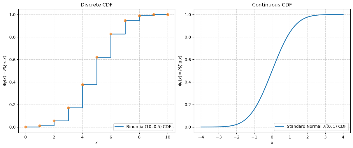

The figure illustrates the fundamental difference between the two cases. In the discrete case, the CDF changes through jumps, while in the continuous case it changes continuously.

Example: Recovering probabilities from a continuous CDF

Suppose that the rotational speed $\xi$ of a shaft is uniformly distributed between 1800 and 2200 revolutions per minute. Its CDF is

\Phi_\xi(x)= \begin{cases} 0, & x<1800,\\ \dfrac{x-1800}{400}, & 1800\leq x\leq2200,\\ 1, & x>2200. \end{cases}

Suppose we want to determine the probability that the rotational speed lies between 1900 and 2000 revolutions per minute. Using the CDF,

\mathbb{P}(\{1900<\xi\leq2000\}) = \Phi_\xi(2000)-\Phi_\xi(1900).

Since

\Phi_\xi(2000)=\frac{2000-1800}{400}=\frac12

and

\Phi_\xi(1900)=\frac{1900-1800}{400}=\frac14,

we obtain

\mathbb{P}(\{1900<\xi\leq2000\}) = \frac12-\frac14 = \frac14.

Because this is a continuous random variable, individual points have probability zero. Consequently, the choice of strict or non-strict inequalities at the endpoints does not affect the result:

\mathbb{P}(\{1900<\xi\leq2000\}) = \mathbb{P}(\{1900\leq\xi\leq2000\}) = \mathbb{P}(\{1900<\xi<2000\}) = \frac14.

Uniform distributions¶

A particularly simple probability distribution is the uniform distribution. It models a situation in which all values in a specified interval are equally likely in the sense that equal-length intervals have equal probability.

A continuous random variable $X$ is said to be uniformly distributed on $[a,b]$ , with $a<b$ , and we write

X\sim U(a,b),

if its density is constant on $[a,b]$ and zero elsewhere. Since the total area under the density must be one,

p_X(x) = \begin{cases} \dfrac{1}{b-a}, & a\leq x\leq b,\\[6pt] 0, & \text{otherwise}. \end{cases}

(4)

For $a\leq x'<x''\leq b$ ,

\mathbb{P}(\{x'<X\leq x''\}) = \int_{x'}^{x''}\frac{1}{b-a}\,dx = \frac{x''-x'}{b-a}.

Thus, for a uniform distribution, the probability of an interval is proportional to its length.

The corresponding CDF is

\Phi_X(x) = \begin{cases} 0, & x<a,\\[4pt] \dfrac{x-a}{b-a}, & a\leq x\leq b,\\[6pt] 1, & x>b. \end{cases}

(5)

The CDF is therefore constant before the interval $[a,b]$ , increases linearly inside the interval, and is equal to one after the interval.

A discrete analogue is obtained by assigning equal probability to a finite set of values. If $X$ takes the $n$ distinct values

x_1,\ldots,x_n

with equal probability, then

\mathbb{P}(\{X=x_i\})=\frac1n, \qquad i=1,\ldots,n.

This is called a discrete uniform distribution.

import matplotlib.pyplot as plt
import numpy as np
from scipy.stats import randint, uniform

fig, axs = plt.subplots(
    2, 2, figsize=(12, 8), layout="constrained"
)

# Continuous Uniform U(a,b)
a, b = 2, 8
x_cont = np.linspace(0, 10, 1000)

pdf_cont = uniform.pdf(x_cont, loc=a, scale=b - a)
cdf_cont = uniform.cdf(x_cont, loc=a, scale=b - a)

axs[0, 0].plot(
    x_cont,
    pdf_cont,
    linewidth=2,
    label=rf"PDF: $\mathcal{{U}}({a},{b})$",
)
axs[0, 0].fill_between(
    x_cont,
    pdf_cont,
    where=(x_cont >= a) & (x_cont <= b),
    alpha=0.2,
)

axs[0, 0].set_title("Continuous Uniform PDF")
axs[0, 0].set_xlabel(r"$x$")
axs[0, 0].set_ylabel(r"$p_X(x)$")
axs[0, 0].set_ylim(-0.02, 0.25)
axs[0, 0].grid(True, linestyle="--", alpha=0.6)
axs[0, 0].legend(loc="upper right")

axs[0, 1].plot(
    x_cont,
    cdf_cont,
    linewidth=2,
    label=rf"CDF: $\mathcal{{U}}({a},{b})$",
)

axs[0, 1].set_title("Continuous Uniform CDF")
axs[0, 1].set_xlabel(r"$x$")
axs[0, 1].set_ylabel(r"$\Phi_X(x)=\mathbb{P}(X\leq x)$")
axs[0, 1].set_ylim(-0.05, 1.05)
axs[0, 1].grid(True, linestyle="--", alpha=0.6)
axs[0, 1].legend(loc="lower right")

# Discrete Uniform distribution: fair die
low, high = 1, 6
x_disc = np.arange(1, 7)
pmf_disc = randint.pmf(x_disc, low, high + 1)

axs[1, 0].stem(
    x_disc,
    pmf_disc,
    linefmt="crimson",
    markerfmt="ro",
    basefmt=" ",
)

axs[1, 0].set_title("Discrete Uniform PMF (Fair Die)")
axs[1, 0].set_xlabel(r"$x$")
axs[1, 0].set_ylabel(r"$P_X(x)$")
axs[1, 0].set_xticks(x_disc)
axs[1, 0].set_ylim(-0.02, 0.25)
axs[1, 0].grid(True, linestyle="--", alpha=0.6)

x_disc_cdf = np.arange(0, 8)
cdf_disc = randint.cdf(x_disc_cdf, low, high + 1)

axs[1, 1].step(
    x_disc_cdf,
    cdf_disc,
    where="post",
    color="crimson",
    linewidth=2,
    label="Discrete CDF",
)
axs[1, 1].plot(x_disc_cdf, cdf_disc, "ro", alpha=0.7)

axs[1, 1].set_title("Discrete Uniform CDF")
axs[1, 1].set_xlabel(r"$x$")
axs[1, 1].set_ylabel(r"$\Phi_X(x)=\mathbb{P}(X\leq x)$")
axs[1, 1].set_ylim(-0.05, 1.05)
axs[1, 1].grid(True, linestyle="--", alpha=0.6)
axs[1, 1].legend(loc="lower right")

plt.show()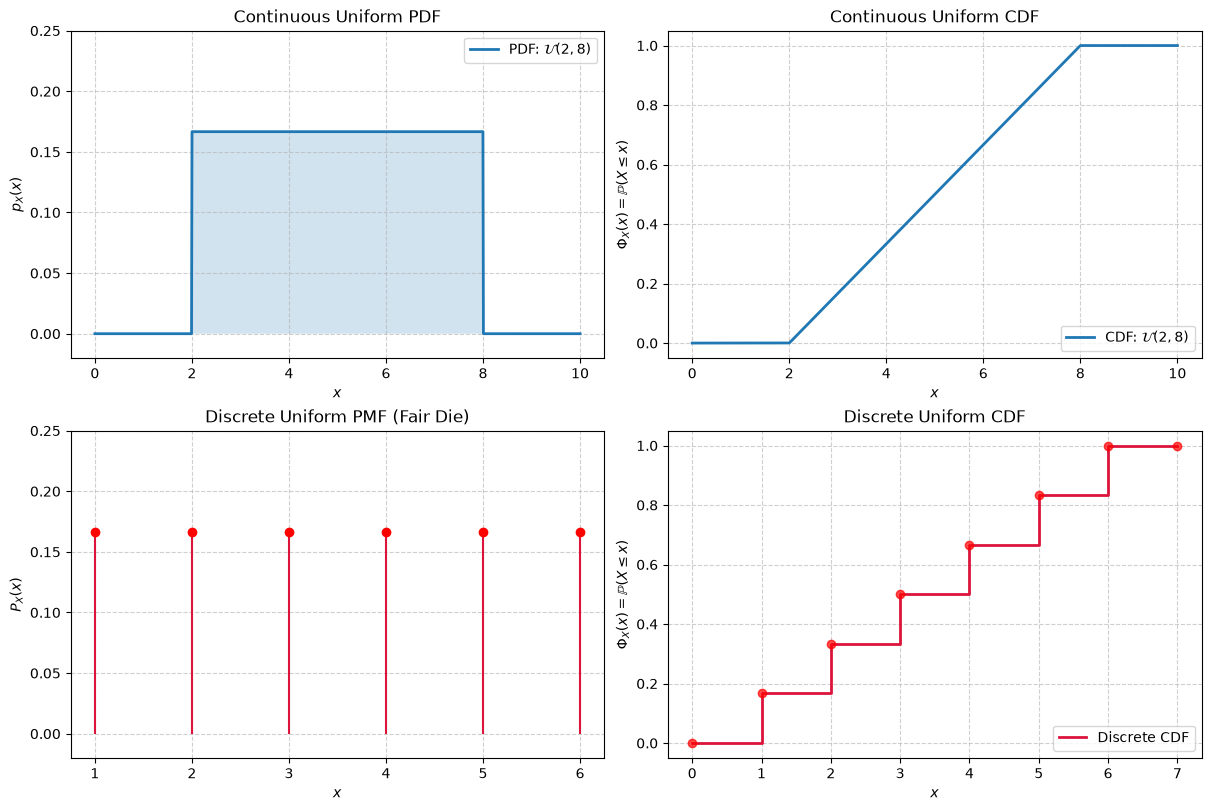

Example: uncertain rotational speed of a mechanical system¶

Random variables are particularly useful for representing uncertain physical quantities.

Suppose that the rotational speed of a shaft varies during operation. Let

\xi=\text{rotational speed of the shaft (rpm)}.

Assume that, during a particular operating regime, the rotational speed can take any value between 1800 rpm and 2200 rpm with equal likelihood. We model this by

\xi\sim U(1800,2200).

Its density is therefore

p_\xi(x) = \begin{cases} \dfrac{1}{400}, & 1800\leq x\leq2200,\\[6pt] 0, & \text{otherwise}. \end{cases}

For example, the probability that the rotational speed lies between 1900 rpm and 2000 rpm is

\begin{aligned} \mathbb{P}(\{1900\leq\xi\leq2000\}) &= \int_{1900}^{2000}p_\xi(x)\,dx\\ &= \frac{1}{400}\int_{1900}^{2000}dx\\ &= \frac{100}{400} = \frac14. \end{aligned}

Thus, under the assumed model, there is a $25\%$ probability that the rotational speed lies between 1900 rpm and 2000 rpm.

The same calculation can be performed directly using the CDF:

\mathbb{P}(\{1900\leq\xi\leq2000\}) = \Phi_\xi(2000)-\Phi_\xi(1900) = \frac{2000-1800}{400} - \frac{1900-1800}{400} = \frac14.

This illustrates the equivalence between the density and CDF descriptions of an absolutely continuous random variable.

Distributions beyond the discrete and continuous cases¶

The discrete and absolutely continuous cases are the two principal settings considered in this course, but they do not exhaust all possible probability distributions.

For example, a random variable may have both discrete and continuous components. Such a distribution is called a mixed distribution.

There are also continuous distribution functions that cannot be represented by an ordinary probability density function. Thus, the statement that a random variable is continuous should not, in complete generality, be taken to mean that it necessarily has a density.

For the purposes of the present course, however, the distinction between discrete random variables described by PMFs and absolutely continuous random variables described by PDFs will cover the main examples and applications.

Example: A mixed random variable

Consider a random variable $\xi$ that takes the value 0 with probability 0.3 and is otherwise uniformly distributed on $(0,1)$ . Its CDF is

\Phi_\xi(x)= \begin{cases} 0, & x<0,\\ 0.3+0.7x, & 0\leq x<1,\\ 1, & x\geq1. \end{cases}

This distribution has both a discrete and a continuous component. In particular, the CDF has a jump of size 0.3 at $x=0$ :

\mathbb{P}(\{\xi=0\}) = \Phi_\xi(0)-\lim_{t\uparrow0}\Phi_\xi(t) = 0.3.

On the other hand, there is no jump at any point $x\in(0,1)$ . For example,

\mathbb{P}(\{\xi=0.5\})=0.

Nevertheless, intervals contained in $(0,1)$ have positive probability. For example,

\mathbb{P}(\{0.2<\xi\leq0.6\}) = \Phi_\xi(0.6)-\Phi_\xi(0.2) = 0.7(0.6-0.2) = 0.28.

This example shows why the CDF is more general than either a probability mass function or a density: it can describe distributions containing both point masses and continuous components.

Summary¶

A random variable assigns a real number to each outcome of a random experiment.

For a discrete random variable, the probability distribution is described by the probability mass function

P_\xi(x)=\mathbb{P}(\{\xi=x\}),

with

\sum_xP_\xi(x)=1.

For an absolutely continuous random variable, the probability distribution is described by a density $p_\xi$ satisfying

p_\xi(x)\geq0, \qquad \int_{-\infty}^{\infty}p_\xi(x)\,dx=1.

Probabilities are obtained by summation in the discrete case and integration in the continuous case.

The cumulative distribution function

\Phi_\xi(x)=\mathbb{P}(\{\xi\leq x\})

provides a unified description of the distribution. In particular,

\mathbb{P}(\{x'<\xi\leq x''\}) = \Phi_\xi(x'')-\Phi_\xi(x').

For a discrete random variable, the CDF is a step function. For a random variable with a density, the CDF is continuous and is obtained by integrating the density.

The next step is to study important families of probability distributions, including the Bernoulli, binomial, Poisson, and normal distributions. These distributions provide models for many common random phenomena and will also provide the foundation for the study of expectation, variance, and limit theorems in the subsequent lectures.