Lecture 4 - Discrete Probability Distributions - Matematica Computazione per L'Ingegneria

In the previous lesson, we introduced random variables and described their probability distributions through probability mass functions, probability density functions, and distribution functions.

In this lesson, we begin a gallery of probability distributions that occur frequently in applications. We first consider discrete random variables. The main examples are the Bernoulli, binomial, geometric, and Poisson distributions.

The expectation and variance of these distributions will be studied systematically in a later lesson. Here we concentrate on understanding how the distributions arise and what their parameters mean.

Bernoulli random variables¶

A Bernoulli experiment is an experiment with two possible outcomes, conventionally called success and failure.

Let $A$ denote the event corresponding to a success. We write

p=\mathbb{P}(A),

and therefore the probability of failure is

q=\mathbb{P}(\overline{A})=1-p.

We assume throughout that

0<p<1.

A Bernoulli random variable $\xi$ is defined by assigning the value 1 to a success and the value 0 to a failure:

\xi= \begin{cases} 1, & \text{with probability }p,\\ 0, & \text{with probability }q. \end{cases}

(1)

Thus, its probability mass function is

P_\xi(k) = \begin{cases} q, & k=0,\\ p, & k=1,\\ 0, & \text{otherwise}. \end{cases}

(2)

We say that $\xi$ has a Bernoulli distribution with parameter $p$ , and write

\xi\sim\operatorname{Bern}(p).

The Bernoulli distribution is the simplest nontrivial discrete probability distribution. It is used whenever an observation can be classified into two possible categories.

For example, a manufactured component may be classified as defective or non-defective, a transmitted bit may be received correctly or incorrectly, or a medical test may produce a positive or negative result.

Repeated Bernoulli trials and the binomial distribution¶

Suppose that the same Bernoulli experiment is repeated $n$ times.

We assume that

the trials are independent;
the probability of success is the same, namely $p$ , in every trial.

Let $\xi_i$ denote the outcome of the $i$ th trial:

\xi_i= \begin{cases} 1, & \text{if the $i$th trial is a success},\\ 0, & \text{if the $i$th trial is a failure}. \end{cases}

The number of successes in the $n$ trials is therefore the random variable

S_n=\xi_1+\cdots+\xi_n.

(3)

The event $\{S_n=k\}$ consists of all sequences of $n$ trials containing exactly $k$ successes and $n-k$ failures.

Consider one particular sequence containing $k$ successes and $n-k$ failures. By independence, its probability is

p^kq^{n-k}.

The number of sequences containing exactly $k$ successes is

\binom{n}{k} = \frac{n!}{k!(n-k)!}.

(4)

Consequently,

\mathbb{P}(\{S_n=k\}) = \binom{n}{k}p^kq^{n-k}, \qquad k=0,1,\ldots,n.

(5)

This is the binomial distribution. We write

S_n\sim\operatorname{Bin}(n,p).

The two parameters have a direct interpretation:

$n$ is the number of trials;
$p$ is the probability of success in each trial.

The binomial distribution therefore models the number of successes obtained in a fixed number of independent and identically distributed Bernoulli trials.

import matplotlib.pyplot as plt
import numpy as np
from scipy.stats import binom

# 1. Define distribution parameters
n = 20  # Total number of trials
p = 0.4  # Probability of success on each trial

# 2. Generate integer k values (from 0 up to n successes)
k = np.arange(0, n + 1)

# 3. Compute PMF and CDF values
pmf_values = binom.pmf(k, n=n, p=p)
cdf_values = binom.cdf(k, n=n, p=p)

# 4. Create side-by-side plots
fig, (ax1, ax2) = plt.subplots(1, 2, figsize=(12, 5))

# Plot 1: Probability Mass Function P(X = k)
ax1.vlines(k, 0, pmf_values, colors='navy', lw=2)
ax1.plot(
    k,
    pmf_values,
    'o',
    color='navy',
    markersize=6,
    label=fr'$\mathrm{{Binom}}(n={n}, p={p})$',
)
ax1.set_title(r'Probability Mass Function $P(X = k)$', fontsize=12)
ax1.set_xlabel('k (number of successes)')
ax1.set_ylabel(r'Probability $P(X = k)$')
ax1.grid(True, linestyle='--', alpha=0.6)
ax1.legend()

# Plot 2: Cumulative Distribution Function F(k)
ax2.step(k, cdf_values, where='post', color='crimson', lw=2, label=r'$F(k)$')
ax2.plot(k, cdf_values, 'o', color='crimson', alpha=0.5, markersize=4)
ax2.set_title(r'Cumulative Distribution Function $F(k)$', fontsize=12)
ax2.set_xlabel('k (number of successes)')
ax2.set_ylabel(r'Probability $F(k)$')
ax2.grid(True, linestyle='--', alpha=0.6)
ax2.legend()

plt.tight_layout()
plt.show()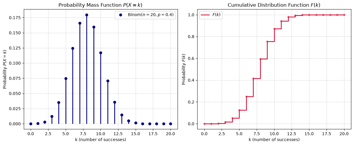

Example: defective components

Suppose that a production process produces components independently, and that each component has probability $p=0.02$ of being defective.

Consider a batch of $n=100$ components, and let $\xi$ denote the number of defective components.

Under the assumptions above,

\xi\sim\operatorname{Bin}(100,0.02).

The probability that exactly five components are defective is

\mathbb{P}(\{\xi=5\}) = \binom{100}{5}(0.02)^5(0.98)^{95}.

Similarly, the probability that no component is defective is

\mathbb{P}(\{\xi=0\}) = (0.98)^{100}.

The binomial model is appropriate because the number of trials is fixed, each trial has two outcomes, and the trials are assumed to be independent with the same probability of success.

The Negative Binomial Distribution¶

Consider again a sequence of independent Bernoulli trials, each with success probability $p$ and failure probability $q = 1 - p$ .

Instead of fixing the total number of trials $n$ in advance, suppose we continue performing trials until a target number $r$ of successes is achieved ( $r \in \{1, 2, 3, \ldots\}$ ).

Let the random variable $X$ denote the number of failures observed before achieving the $r$ th success.

The event $\{X = k\}$ means that:

the $(r + k)$ th trial is the $r$ th success;
among the first $r + k - 1$ trials, there are exactly $r - 1$ successes and $k$ failures.

By independence of the trials, the probability of any specific sequence of $r+k$ trials containing $r$ successes and $k$ failures with a success at the final trial is

p^r q^k.

The number of ways to choose the positions of the first $r-1$ successes among the first $r+k-1$ trials is given by the binomial coefficient

\binom{r+k-1}{r-1} = \binom{r+k-1}{k}.

(6)

Consequently, the probability mass function of $X$ is

\mathbb{P}(\{X = k\}) = \binom{k+r-1}{k} p^r q^k, \qquad k = 0, 1, 2, \ldots

(7)

This is the negative binomial distribution. We write

X \sim \operatorname{NB}(r, p).

The two parameters have a direct interpretation:

$r$ is the target number of successes;
$p$ is the probability of success in each trial.

The negative binomial distribution therefore models the number of failures encountered before obtaining a fixed number $r$ of successes in independent and identically distributed Bernoulli trials.

import matplotlib.pyplot as plt
import numpy as np
from scipy.stats import nbinom

# 1. Define distribution parameters
r = 5   # Target number of successes
p = 0.4 # Probability of success on each trial

# 2. Generate integer k values (number of failures before r successes)
k = np.arange(0, 25)

# 3. Compute PMF and CDF values
pmf_values = nbinom.pmf(k, n=r, p=p)
cdf_values = nbinom.cdf(k, n=r, p=p)

# 4. Create side-by-side plots
fig, (ax1, ax2) = plt.subplots(1, 2, figsize=(12, 5))

# Plot 1: Probability Mass Function P(X = k)
ax1.vlines(k, 0, pmf_values, colors='navy', lw=2)
ax1.plot(
    k,
    pmf_values,
    'o',
    color='navy',
    markersize=6,
    label=fr'$\mathrm{{NBinom}}(r={r}, p={p})$',
)
ax1.set_title(r'Probability Mass Function $P(X = k)$', fontsize=12)
ax1.set_xlabel('k (number of failures)')
ax1.set_ylabel(r'Probability $P(X = k)$')
ax1.grid(True, linestyle='--', alpha=0.6)
ax1.legend()

# Plot 2: Cumulative Distribution Function F(k)
ax2.step(k, cdf_values, where='post', color='crimson', lw=2, label=r'$F(k)$')
ax2.plot(k, cdf_values, 'o', color='crimson', alpha=0.5, markersize=4)
ax2.set_title(r'Cumulative Distribution Function $F(k)$', fontsize=12)
ax2.set_xlabel('k (number of failures)')
ax2.set_ylabel(r'Probability $F(k)$')
ax2.grid(True, linestyle='--', alpha=0.6)
ax2.legend()

plt.tight_layout()
plt.show()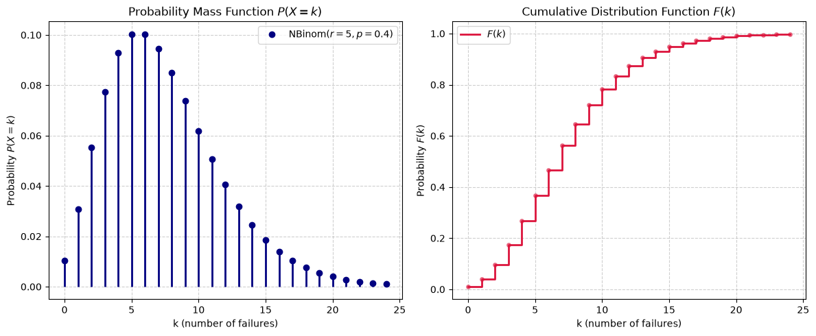

Example: testing till defect quota

Suppose components from a production process are tested sequentially until $r = 3$ non-defective components are produced.

Each component is non-defective (success) with probability $p = 0.8$ , independently of the others.Let $\xi$ denote the number of defective components (failures) observed before obtaining the 3rd non-defective component.

Under the assumptions above,

\xi \sim \operatorname{NB}(3, 0.8).

The probability that exactly two defective components are produced before getting three non-defective ones is

\mathbb{P}({\xi = 2}) = \binom{2 + 3 - 1}{2} (0.8)^3 (0.2)^2 = \binom{4}{2} (0.8)^3 (0.2)^2 = 0.12288.

Similarly, the probability of obtaining three non-defective components without encountering any defective ones is

\mathbb{P}({\xi = 0}) = (0.8)^3 = 0.512.

Example: Mechanical engineering component fatigue

Consider a fatigue testing process in mechanical engineering where structural fasteners are subjected to repeated cyclic stress until micro-cracks develop.

Suppose that during each load cycle, the probability of initiating a micro-crack is $p = 0.002$ , with cycles assumed to be independent. Testing continues until $r = 2$ micro-cracks are observed to evaluate material endurance.

Let $\xi$ denote the number of un-cracked load cycles observed before achieving the target of 2 micro-cracks.

Under these assumptions,

\xi \sim \operatorname{NB}(2, 0.002).

The probability that a component survives exactly 1000 un-cracked cycles before developing its second micro-crack is

\begin{split} \mathbb{P}(\{\xi = 1000\}) = & \binom{1000 + 2 - 1}{1000} (0.002)^2 (0.998)^{1000} \\ = & 1001 \cdot (0.002)^2 \cdot (0.998)^{1000} \approx 0.00054. \end{split}

This negative binomial model allows mechanical engineers to estimate component reliability, set maintenance schedules, and evaluate safety margins for structural elements under fatigue loading.

The geometric distribution¶

The binomial distribution counts the number of successes in a fixed number of trials.

A different question is obtained when we continue performing independent Bernoulli trials until the first success occurs.

Let $\xi$ denote the number of trials required to obtain the first success.

For $\xi$ to take the value $k$ , the first $k-1$ trials must all be failures and the $k$ th trial must be a success. Therefore,

\mathbb{P}(\{\xi=k\}) = q^{k-1}p, \qquad k=1,2,3,\ldots.

Thus, the probability mass function is

P_\xi(k) = p(1-p)^{k-1}, \qquad k=1,2,3,\ldots.

(8)

This is called the geometric distribution with parameter $p$ , and we write

\xi\sim\operatorname{Geom}(p).

The geometric distribution is therefore a waiting-time distribution: it describes how many independent Bernoulli trials are needed before the first success.

For example, if a communication system successfully transmits a packet with probability $p=0.9$ at every attempt, then the number of attempts required for the first successful transmission has a geometric distribution.

The first few probabilities are

\begin{aligned} \mathbb{P}(\{\xi=1\}) &=p,\\ \mathbb{P}(\{\xi=2\}) &=qp,\\ \mathbb{P}(\{\xi=3\}) &=q^2p,\\ \mathbb{P}(\{\xi=4\}) &=q^3p. \end{aligned}

The probabilities decrease geometrically as the waiting time increases.

The distribution is correctly normalized because

\sum_{k=1}^{\infty}p(1-p)^{k-1} = p\sum_{j=0}^{\infty}q^j = \frac{p}{1-q} = 1.

import matplotlib.pyplot as plt
import numpy as np
from scipy.stats import geom

# 1. Define distribution parameter
p = 0.3  # Probability of success on each trial

# 2. Generate integer k values starting from 1 (first success)
# Range set to cover ~99.9% of the distribution tail
k_max = int(geom.ppf(0.999, p))
k = np.arange(1, k_max + 1)

# 3. Compute PMF and CDF values
pmf_values = geom.pmf(k, p=p)
cdf_values = geom.cdf(k, p=p)

# 4. Create side-by-side plots
fig, (ax1, ax2) = plt.subplots(1, 2, figsize=(12, 5))

# Plot 1: Probability Mass Function P(X = k)
ax1.vlines(k, 0, pmf_values, colors='navy', lw=2)
ax1.plot(
    k,
    pmf_values,
    'o',
    color='navy',
    markersize=6,
    label=fr'$\mathrm{{Geom}}(p={p})$',
)
ax1.set_title(r'Probability Mass Function $P(X = k)$', fontsize=12)
ax1.set_xlabel('k (number of trials)')
ax1.set_ylabel(r'Probability $P(X = k)$')
ax1.grid(True, linestyle='--', alpha=0.6)
ax1.legend()

# Plot 2: Cumulative Distribution Function F(k)
ax2.step(k, cdf_values, where='post', color='crimson', lw=2, label=r'$F(k)$')
ax2.plot(k, cdf_values, 'o', color='crimson', alpha=0.5, markersize=4)
ax2.set_title(r'Cumulative Distribution Function $F(k)$', fontsize=12)
ax2.set_xlabel('k (number of trials)')
ax2.set_ylabel(r'Probability $F(k)$')
ax2.grid(True, linestyle='--', alpha=0.6)
ax2.legend()

plt.tight_layout()
plt.show()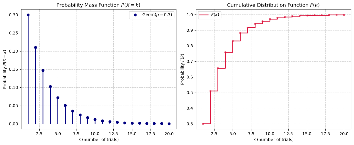

The Poisson distribution¶

The binomial distribution describes the number of successes in a fixed number of trials.

There are situations, however, in which events are naturally described as rare occurrences over a large number of opportunities. Examples include:

defects in a large production batch;
failures of components during a fixed period of operation;
calls arriving at a service centre;
accidents occurring along a stretch of road;
radioactive decay events during a fixed time interval.

Suppose that

n\to\infty, \qquad p\to0, \qquad np\to a>0.

Thus, the number of opportunities becomes large, the probability of success at each opportunity becomes small, while the expected number of successes remains of order one.

In this regime, the binomial distribution approaches the Poisson distribution.

For fixed $k$ ,

\lim_{n\to\infty} \binom{n}{k}p^k(1-p)^{n-k} = \frac{a^k}{k!}e^{-a}.

(9)

This motivates the following definition.

The parameter $a$ represents the typical number of occurrences in the interval, region, or population being considered. The fact that the same parameter will later turn out to be both the mean and the variance will be derived when moments are studied.

import matplotlib.pyplot as plt
import numpy as np
from scipy.stats import poisson

# 1. Define distribution parameter
lam = 5  # Lambda (average rate / mean)

# 2. Generate integer x values (Poisson is non-negative and discrete)
# We cover roughly 4 standard deviations (std = sqrt(lambda))
x_max = int(lam + 4 * np.sqrt(lam)) + 1
x = np.arange(0, x_max)

# 3. Compute PMF and CDF values
pmf_values = poisson.pmf(x, mu=lam)
cdf_values = poisson.cdf(x, mu=lam)

# 4. Create side-by-side plots
fig, (ax1, ax2) = plt.subplots(1, 2, figsize=(12, 5))

# Plot 1: Probability Mass Function P(X = k)
ax1.vlines(x, 0, pmf_values, colors='navy', lw=2)
ax1.plot(
    x,
    pmf_values,
    'o',
    color='navy',
    markersize=6,
    label=fr'$\mathrm{{Poisson}}(\lambda={lam})$',
)
ax1.set_title(r'Probability Mass Function $P(X = k)$', fontsize=12)
ax1.set_xlabel('k')
ax1.set_ylabel(r'Probability $P(X = k)$')
ax1.grid(True, linestyle='--', alpha=0.6)
ax1.legend()

# Plot 2: Cumulative Distribution Function F(k)
ax2.step(x, cdf_values, where='post', color='crimson', lw=2, label=r'$F(k)$')
ax2.plot(x, cdf_values, 'o', color='crimson', alpha=0.5, markersize=4)
ax2.set_title(r'Cumulative Distribution Function $F(k)$', fontsize=12)
ax2.set_xlabel('k')
ax2.set_ylabel(r'Probability $F(k)$')
ax2.grid(True, linestyle='--', alpha=0.6)
ax2.legend()

plt.tight_layout()
plt.show()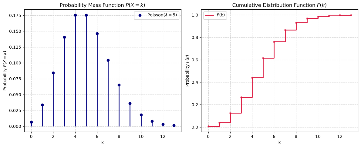

Why does the Poisson formula arise?¶

The connection with the binomial distribution can be seen directly.

Suppose that $p=a/n$ . Then

\mathbb{P}(\{S_n=k\}) = \binom{n}{k} \left(\frac{a}{n}\right)^k \left(1-\frac{a}{n}\right)^{n-k}.

For fixed $k$ ,

\binom{n}{k} \left(\frac{a}{n}\right)^k = \frac{a^k}{k!} \frac{n(n-1)\cdots(n-k+1)}{n^k} \longrightarrow \frac{a^k}{k!},

while

\left(1-\frac{a}{n}\right)^n \longrightarrow e^{-a},

and

\left(1-\frac{a}{n}\right)^{-k} \longrightarrow1.

Combining these limits gives (7).

Thus, the Poisson distribution can be regarded as the limiting model for a large number of independent trials with a small probability of success.

Poisson model for bearing defects

Consider a manufacturing process in which bearings are produced continuously. Suppose that, on average, 2 defective bearings are found in a batch of 1000 bearings.

If defects are rare and their occurrences can reasonably be regarded as independent, it is natural to use a Poisson model with parameter $a=2$ .

Let $\xi$ denote the number of defective bearings in a batch. Then

\xi\sim\operatorname{Pois}(2).

The probability of observing no defective bearings is

\mathbb{P}(\{\xi=0\}) = e^{-2} \approx0.1353.

The probability of observing exactly three defective bearings is

\mathbb{P}(\{\xi=3\}) = \frac{2^3}{3!}e^{-2} \approx0.1804.

The probability of finding at most two defective bearings is

\begin{aligned} \mathbb{P}(\{\xi\leq2\}) &= \sum_{k=0}^{2}\frac{2^k}{k!}e^{-2}\\ &= e^{-2} \left( 1+2+\frac{2^2}{2!} \right)\\ &= 5e^{-2}\\ &\approx0.6767. \end{aligned}

The Poisson model is appropriate here because the number of opportunities is large, defects are relatively rare, and the average number of defects remains finite.

The Compound Poisson Distribution¶

In many practical situations, we are interested not only in the number of events that occur, but also in the total accumulated value associated with those events. Examples include:

the total monetary amount of insurance claims filed in a year (where $N$ is the number of claims and $X_i$ is the claim size);
the total amount of rainfall in a region (where $N$ is the number of storms and $X_i$ is the rainfall per storm);
the total expenditure of customers in a store (where $N$ is the number of customers and $X_i$ is the amount spent by the $i$ th customer).

This naturally leads to the concept of a compound Poisson distribution.

The parameter $a$ represents the expected frequency of events, while the distribution of $X_i$ models the random severity or size of each individual event.

import matplotlib.pyplot as plt
import numpy as np

# 1. Define distribution parameters
a = 10  # Expected number of events N ~ Pois(a)
num_samples = 100000

# 2. Simulate N and claim sizes X_i
np.random.seed(42)
N_samples = np.random.poisson(lam=a, size=num_samples)

# Suppose each X_i is discrete with values {10, 20, 50} and probabilities [0.5, 0.3, 0.2]
x_vals = np.array([10, 20, 50])
x_probs = np.array([0.5, 0.3, 0.2])

S_samples = np.zeros(num_samples)
for i in range(num_samples):
    if N_samples[i] > 0:
        S_samples[i] = np.sum(np.random.choice(x_vals, size=N_samples[i], p=x_probs))

# 3. Create side-by-side plots
fig, (ax1, ax2) = plt.subplots(1, 2, figsize=(12, 5))

# Plot 1: Simulated Distribution Histogram
ax1.hist(S_samples, bins=40, density=True, color='navy', alpha=0.7, edgecolor='black')
ax1.set_title(r'Simulated Compound Poisson PMF/Density', fontsize=12)
ax1.set_xlabel('Total Sum $S$')
ax1.set_ylabel('Probability Density')
ax1.grid(True, linestyle='--', alpha=0.6)

# Plot 2: Empirical Cumulative Distribution Function
sorted_S = np.sort(S_samples)
cdf_empirical = np.arange(1, num_samples + 1) / num_samples
ax2.plot(sorted_S, cdf_empirical, color='crimson', lw=2, label=r'Empirical $F(S)$')
ax2.set_title(r'Empirical Cumulative Distribution Function $F(S)$', fontsize=12)
ax2.set_xlabel('Total Sum $S$')
ax2.set_ylabel(r'Probability $F(S)$')
ax2.grid(True, linestyle='--', alpha=0.6)
ax2.legend()

plt.tight_layout()
plt.show()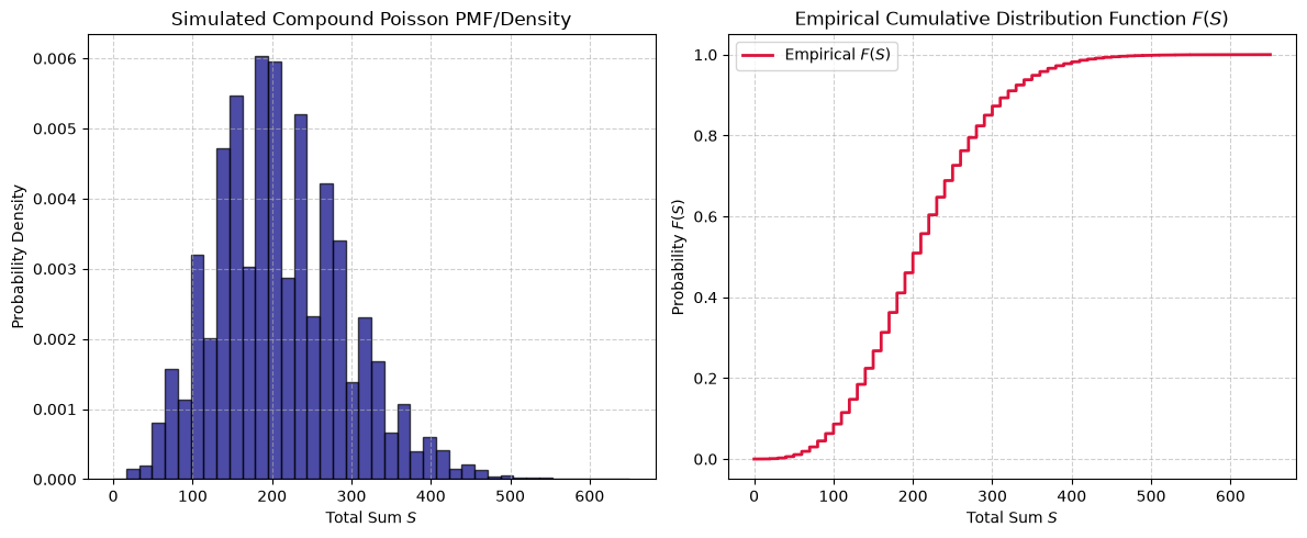

Example: Hydraulic pipeline pressure surges

Consider a hydraulic system in heavy machinery subject to transient pressure spikes (water hammer events) caused by sudden valve closures.

Suppose the number of pressure spikes $N$ occurring during a 100-hour operating period follows a Poisson distribution with an average rate of $a = 4$ events, so $N \sim \operatorname{Pois}(4)$ .

Each individual pressure surge induces a random increment of mechanical stress $X_i$ (in MPa) on the pipe wall. Assume each $X_i$ is independent and takes a value of either $20\text{ MPa}$ (with probability 0.8) or $50\text{ MPa}$ (with probability 0.2).

The total accumulated stress load $S$ over the 100-hour period is given by the compound Poisson sum:

S = \sum_{i=1}^{N} X_i.

If no pressure surges occur during operation ( $N = 0$ ), the total added stress load is $S = 0$ , which occurs with probability:

\mathbb{P}(\{S = 0\}) = \mathbb{P}(\{N = 0\}) = e^{-4} \approx 0.0183.

The compound Poisson model allows mechanical engineers to evaluate the cumulative fatigue damage on pressure vessels and piping by accounting for both the random frequency $N$ of transient events and the random severity $X_i$ of each event.

The Mixed Poisson Distribution¶

In the standard Poisson model, the rate parameter $a$ is assumed to be constant across all observations. In many engineering and real-world applications, however, environmental conditions, operational stress, or batch-to-batch material variations cause the underlying intensity parameter to fluctuate randomly from one system or time window to another.

This leads to the mixed Poisson distribution (or Poisson mixture), where the intensity parameter itself is modeled as a non-negative random variable $\Lambda$ .

Definition 3 (Mixed Poisson distribution)

Let $\Lambda$ be a non-negative continuous random variable with probability density function $g(\lambda)$ . A non-negative integer-valued random variable $\xi$ has a mixed Poisson distribution with mixing density $g(\lambda)$ if, conditionally on $\Lambda = \lambda$ , $\xi \sim \operatorname{Pois}(\lambda)$ :

\mathbb{P}(\{\xi = k\} \mid \Lambda = \lambda) = \frac{\lambda^k}{k!} e^{-\lambda}, \qquad k = 0, 1, 2, \ldots

The unconditional probability mass function of $\xi$ is obtained by integrating over all possible values of $\lambda$ :

\mathbb{P}(\{\xi = k\}) = \int_{0}^{\infty} \frac{\lambda^k}{k!} e^{-\lambda} g(\lambda) \, d\lambda, \qquad k = 0, 1, 2, \ldots

(12)

The mixing distribution $g(\lambda)$ represents the uncertainty or population heterogeneity in the event rate across different operating environments.

import matplotlib.pyplot as plt
import numpy as np
from scipy.stats import gamma, poisson

# 1. Define mixing distribution parameters (Gamma distribution for rate Lambda)
shape = 3.0  # Gamma shape parameter r
scale = 1.5  # Gamma scale parameter theta

# 2. Generate grid of k values
k_vals = np.arange(0, 25)

# 3. Numerically evaluate unconditional PMF P(X = k)
pmf_mixed = np.zeros_like(k_vals, dtype=float)
for i, k in enumerate(k_vals):
    # Integrand: Pois(k | lambda) * Gamma(lambda)
    integrand = lambda lam: poisson.pmf(k, mu=lam) * gamma.pdf(lam, a=shape, scale=scale)
    # Integrate over lambda in [0, inf)
    from scipy.integrate import quad
    pmf_mixed[i], _ = quad(integrand, 0, np.inf)

# 4. Plot Mixed Poisson PMF
plt.figure(figsize=(7, 4.5))
plt.vlines(k_vals, 0, pmf_mixed, colors='navy', lw=2)
plt.plot(k_vals, pmf_mixed, 'o', color='navy', markersize=6, label=r'Mixed Poisson ($\Lambda \sim \mathrm{Gamma}$)')
plt.title(r'Probability Mass Function of Mixed Poisson Distribution', fontsize=12)
plt.xlabel('k (number of events)')
plt.ylabel(r'Probability $P(\xi = k)$')
plt.grid(True, linestyle='--', alpha=0.6)
plt.legend()
plt.tight_layout()
plt.show()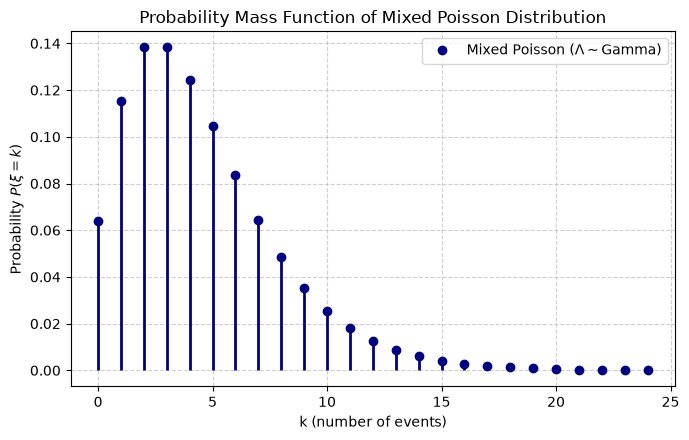

Comparing the discrete distributions¶

The distributions introduced in this lesson describe different types of counting problems.

Distribution	Random quantity	Parameters	Typical question
Bernoulli	One success/failure outcome	$p$	Does the event occur?
Binomial	Number of successes in $n$ trials	$n,p$	How many successes occur?
Geometric	Number of trials before first success	$p$	How long until the first success?
Negative Binomial	Number of failures before $r$ successes	$r,p$	How many failures occur before a given number of successes?
Poisson	Number of rare events	$a$	How many events occur in a given interval?

The relationships between these distributions are particularly important.

A Bernoulli random variable represents a single trial. The binomial distribution counts successes in a fixed number of independent Bernoulli trials. The geometric distribution instead counts how many trials are needed to obtain the first success, while the negative binomial distribution generalizes this to count failures before achieving a target number $r$ of successes. Finally, the Poisson distribution arises as a limiting model for rare successes when the number of opportunities is large.

These distinctions are often more important in applications than the formulas themselves: choosing a probability distribution means identifying the random mechanism that generates the observations.

A short computational illustration¶

The binomial and Poisson distributions can be compared when $n$ is large and $p$ is small.

For example, consider

n=1000, \qquad p=0.002,

so that

np=2.

The corresponding binomial distribution is therefore expected to be close to a Poisson distribution with parameter $a=2$ .

import numpy as np
import matplotlib.pyplot as plt
from scipy.stats import binom, poisson

n = 1000
p = 0.002
a = n * p

k = np.arange(0, 12)

binomial_pmf = binom.pmf(k, n, p)
poisson_pmf = poisson.pmf(k, a)

plt.figure(figsize=(8, 5))

plt.plot(
    k,
    binomial_pmf,
    "o-",
    label=r"$\operatorname{Bin}(1000,0.002)$"
)

plt.plot(
    k,
    poisson_pmf,
    "s--",
    label=r"$\operatorname{Pois}(2)$"
)

plt.xlabel("Number of successes")
plt.ylabel("Probability")
plt.title("Binomial distribution and Poisson approximation")
plt.grid(True, alpha=0.3)
plt.legend()
plt.show()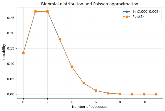

The two distributions are very close in this example. This illustrates why the Poisson distribution is useful: it can replace a binomial model when $n$ is large and $p$ is small, while keeping the average number of successes $np$ fixed.

Summary¶

The main discrete probability distributions introduced in this lesson are:

Bernoulli: one trial with two possible outcomes; Binomial: the number of successes in a fixed number of independent Bernoulli trials; Geometric: the number of trials required to obtain the first success; Poisson: the number of rare events occurring in a specified setting.

The binomial and Poisson distributions are connected by the rare-event limit

n\to\infty, \qquad p\to0, \qquad np\to a.

In the next lesson we turn to important continuous probability distributions, in particular the uniform, exponential, and normal distributions. We will also see how the normal distribution emerges as a limit of the binomial distribution, providing the first step toward the central limit theorem.