Lecture 5 - Continuous Probability Distributions - Matematica Computazione per L'Ingegneria

Continuous Probability Distributions¶

In the previous lecture, we introduced several important discrete probability distributions, including the Bernoulli, binomial, geometric, and Poisson distributions. These distributions are appropriate when the possible outcomes form a finite or countable set.

Many quantities arising in applications, however, can take values in a continuum. Examples include:

the lifetime of a component;
the diameter of a manufactured part;
the temperature of a system;
the measurement error of an instrument;
the time between successive events.

Such quantities are modeled by continuous random variables.

In this lecture we introduce several important continuous distributions and, in particular, the normal distribution, which plays a central role in probability and statistics.

We will also see that the normal distribution naturally arises as an approximation to the binomial distribution when the number of trials is large. This provides our first connection between discrete probability distributions and continuous probability distributions.

Continuous probability distributions¶

Recall from Lecture 3 that a continuous random variable $\xi$ is described by a probability density function $p_\xi$ , satisfying

p_\xi(x)\geq 0, \qquad \int_{-\infty}^{+\infty}p_\xi(x)\,dx=1.

The probability that $\xi$ belongs to an interval is obtained by integrating the density over that interval:

\mathbb{P}(\{a<\xi\leq b\}) = \int_a^b p_\xi(x)\,dx.

(1)

In particular, the probability that a continuous random variable takes one particular value is zero:

\mathbb{P}(\{\xi=x\})=0.

Therefore, for continuous random variables, the distinction between open and closed endpoints does not affect interval probabilities:

\mathbb{P}(\{a<\xi<b\}) = \mathbb{P}(\{a\leq\xi\leq b\}).

The cumulative distribution function is

F_\xi(x) = \mathbb{P}(\{\xi\leq x\}) = \int_{-\infty}^x p_\xi(t)\,dt.

(2)

Whenever $F_\xi$ is differentiable,

p_\xi(x)=F_\xi'(x).

The density should not be interpreted as a probability assigned to a single point. Rather, it determines probabilities through integration.

The uniform distribution¶

The simplest continuous distribution is the uniform distribution.

A random variable $\xi$ is uniformly distributed on the interval $[a,b]$ , with $a<b$ , if its density is constant on that interval and zero elsewhere:

p_\xi(x) = \begin{cases} \dfrac{1}{b-a}, & a\leq x\leq b,\\[6pt] 0, & \text{otherwise}. \end{cases}

(3)

We write

\xi\sim U(a,b).

The normalization condition follows immediately:

\int_{-\infty}^{+\infty}p_\xi(x)\,dx = \int_a^b\frac{1}{b-a}\,dx = 1.

The probability of an interval contained in $[a,b]$ is proportional to its length. In particular, if $a\leq c\leq d\leq b$ ,

\mathbb{P}(\{c\leq\xi\leq d\}) = \frac{d-c}{b-a}.

(4)

The cumulative distribution function is

F_\xi(x) = \begin{cases} 0, & x<a,\\[4pt] \dfrac{x-a}{b-a}, & a\leq x\leq b,\\[8pt] 1, & x>b. \end{cases}

(5)

import matplotlib.pyplot as plt
import numpy as np
from scipy.stats import uniform

# 1. Define distribution parameters
a = 0  # Lower bound
b = 10  # Upper bound
scale = b - a  # Interval width (scipy scale parameter)

# 2. Generate x values extending slightly beyond [a, b]
padding = scale * 0.25
x = np.linspace(a - padding, b + padding, 1000)

# 3. Compute PDF and CDF values
pdf_values = uniform.pdf(x, loc=a, scale=scale)
cdf_values = uniform.cdf(x, loc=a, scale=scale)

# 4. Create side-by-side plots
fig, (ax1, ax2) = plt.subplots(1, 2, figsize=(12, 5))

# Plot 1: Probability Density Function f(x)
ax1.plot(x, pdf_values, color='navy', lw=2, label=fr'$\mathcal{{U}}({a}, {b})$')
ax1.fill_between(x, pdf_values, color='skyblue', alpha=0.4)
ax1.set_title(r'Probability Density Function $f(x)$', fontsize=12)
ax1.set_xlabel('x')
ax1.set_ylabel(r'Density $f(x)$')
ax1.grid(True, linestyle='--', alpha=0.6)
ax1.legend()

# Plot 2: Cumulative Distribution Function F(x)
ax2.plot(x, cdf_values, color='crimson', lw=2, label=r'$F(x)$')
ax2.set_title(r'Cumulative Distribution Function $F(x)$', fontsize=12)
ax2.set_xlabel('x')
ax2.set_ylabel(r'Probability $F(x)$')
ax2.grid(True, linestyle='--', alpha=0.6)
ax2.legend()

plt.tight_layout()
plt.show()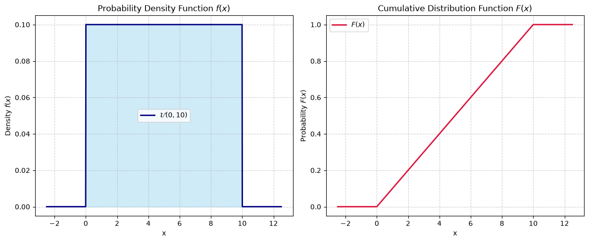

The exponential distribution¶

The exponential distribution is particularly useful for modeling waiting times.

A random variable $\xi$ has an exponential distribution with parameter $\lambda>0$ if its density is

p_\xi(x) = \begin{cases} \lambda e^{-\lambda x}, & x\geq0,\\ 0, & x<0. \end{cases}

(6)

We write

\xi\sim\operatorname{Exp}(\lambda).

The normalization follows from

\int_0^\infty\lambda e^{-\lambda x}\,dx = 1.

The cumulative distribution function is

F_\xi(x) = \begin{cases} 0, & x<0,\\[4pt] 1-e^{-\lambda x}, & x\geq0. \end{cases}

(7)

Consequently,

\mathbb{P}(\{\xi>t\}) = e^{-\lambda t}, \qquad t\geq0.

(8)

The parameter $\lambda$ is a rate parameter. A larger value of $\lambda$ corresponds to shorter typical waiting times.

import matplotlib.pyplot as plt
import numpy as np
from scipy.stats import expon

# 1. Define distribution parameter
rate = 0.5  # Rate parameter lambda
scale = 1 / rate  # Scale parameter (1/lambda = mean)

# 2. Generate x values across 4 standard deviations (std = scale = 1/lambda)
x = np.linspace(0, 4 * scale, 1000)

# 3. Compute PDF and CDF values
pdf_values = expon.pdf(x, scale=scale)
cdf_values = expon.cdf(x, scale=scale)

# 4. Create side-by-side plots
fig, (ax1, ax2) = plt.subplots(1, 2, figsize=(12, 5))

# Plot 1: Probability Density Function f(x)
ax1.plot(
    x,
    pdf_values,
    color='navy',
    lw=2,
    label=fr'$\mathrm{{Exp}}(\lambda={rate})$',
)
ax1.fill_between(x, pdf_values, color='skyblue', alpha=0.4)
ax1.set_title(r'Probability Density Function $f(x)$', fontsize=12)
ax1.set_xlabel('x')
ax1.set_ylabel(r'Density $f(x)$')
ax1.grid(True, linestyle='--', alpha=0.6)
ax1.legend()

# Plot 2: Cumulative Distribution Function F(x)
ax2.plot(x, cdf_values, color='crimson', lw=2, label=r'$F(x)$')
ax2.set_title(r'Cumulative Distribution Function $F(x)$', fontsize=12)
ax2.set_xlabel('x')
ax2.set_ylabel(r'Probability $F(x)$')
ax2.grid(True, linestyle='--', alpha=0.6)
ax2.legend()

plt.tight_layout()
plt.show()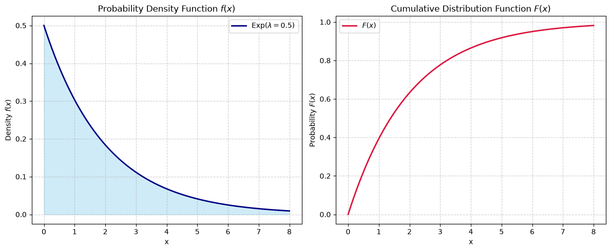

The memoryless property

The exponential distribution has an important property known as memorylessness.

For $s,t\geq0$ ,

\mathbb{P}(\{\xi>s+t\}\mid\{\xi>s\}) = \mathbb{P}(\{\xi>t\}).

(9)

Indeed,

\begin{aligned} \mathbb{P}(\{\xi>s+t\}\mid\{\xi>s\}) &= \frac{\mathbb{P}(\{\xi>s+t\})} {\mathbb{P}(\{\xi>s\})}\\ &= \frac{e^{-\lambda(s+t)}}{e^{-\lambda s}}\\ &= e^{-\lambda t}. \end{aligned}

Thus, conditional on having already waited $s$ units of time, the additional waiting time has the same distribution as the original waiting time.

This property is one reason why exponential random variables arise naturally in models of random arrivals and failures.

The normal distribution¶

Among continuous probability distributions, the normal distribution is perhaps the most important.

It is used to model measurement errors, physical quantities subject to many small random effects, and numerous quantities arising from aggregation and averaging.

The standard normal density is

\varphi(x) = \frac{1}{\sqrt{2\pi}} e^{-x^2/2}, \qquad x\in\mathbb{R}.

(10)

The corresponding random variable is said to have a standard normal distribution, denoted by

\xi\sim N(0,1).

The density is symmetric about $x=0$ :

\varphi(-x)=\varphi(x).

It has its maximum at $x=0$ and decreases rapidly as $|x|$ increases.

The constant $\sqrt{2\pi}$ is chosen so that

\int_{-\infty}^{+\infty} \frac{1}{\sqrt{2\pi}}e^{-x^2/2}\,dx = 1.

(11)

The cumulative distribution function of the standard normal distribution is denoted by $\Phi$ :

\Phi(x) = \mathbb{P}(\{\xi\leq x\}) = \frac{1}{\sqrt{2\pi}} \int_{-\infty}^x e^{-t^2/2}\,dt.

(12)

There is no elementary antiderivative for $e^{-x^2/2}$ . Consequently, values of $\Phi$ are normally computed using tables, numerical algorithms, or software.

By symmetry,

\Phi(-x)=1-\Phi(x).

(13)

This identity is particularly useful when computing normal probabilities.

import matplotlib.pyplot as plt
import numpy as np
from scipy.stats import norm

# 1. Define standard normal distribution parameters
mu = 0  # Mean
sigma = 1  # Standard deviation

# 2. Generate x values across 4 standard deviations
x = np.linspace(-4, 4, 1000)

# 3. Compute PDF and CDF values
pdf_values = norm.pdf(x, loc=mu, scale=sigma)
cdf_values = norm.cdf(x, loc=mu, scale=sigma)

# 4. Create side-by-side plots
fig, (ax1, ax2) = plt.subplots(1, 2, figsize=(12, 5))

# Plot 1: Probability Density Function \phi(z)
ax1.plot(
    x,
    pdf_values,
    color='navy',
    lw=2,
    label=r'$\mathcal{N}(0, 1)$',
)
ax1.fill_between(x, pdf_values, color='skyblue', alpha=0.4)
ax1.set_title(r'Probability Density Function $\phi(z)$', fontsize=12)
ax1.set_xlabel('z')
ax1.set_ylabel(r'Density $\phi(z)$')
ax1.grid(True, linestyle='--', alpha=0.6)
ax1.legend()

# Plot 2: Cumulative Distribution Function \Phi(z)
ax2.plot(x, cdf_values, color='crimson', lw=2, label=r'$\Phi(z)$')
ax2.set_title(r'Cumulative Distribution Function $\Phi(z)$', fontsize=12)
ax2.set_xlabel('z')
ax2.set_ylabel(r'Probability $\Phi(z)$')
ax2.grid(True, linestyle='--', alpha=0.6)
ax2.legend()

plt.tight_layout()
plt.show()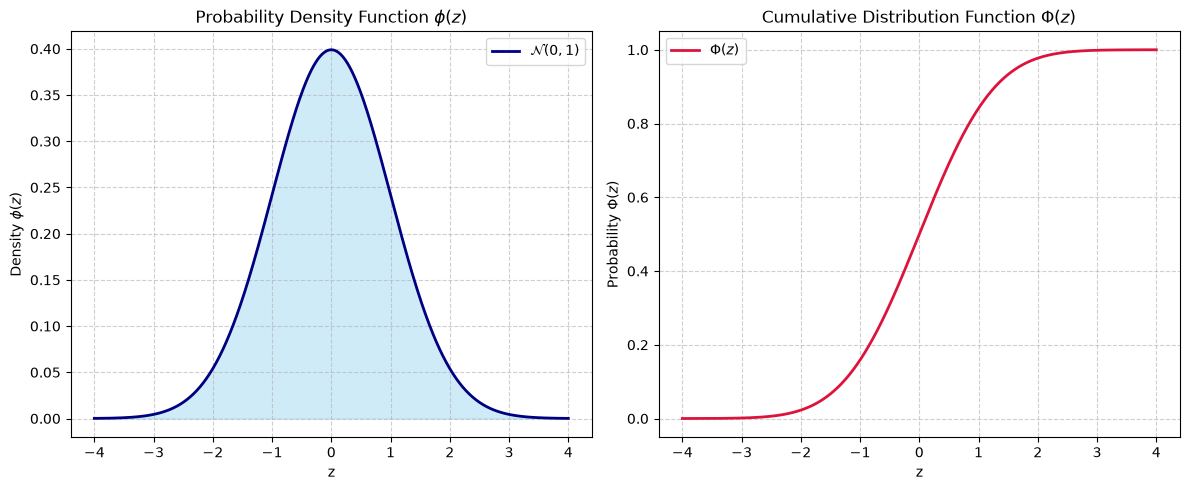

The general normal distribution¶

The standard normal distribution can be shifted and rescaled.

Let

\xi=a+\sigma Z,

where

Z\sim N(0,1), \qquad \sigma>0.

Then $\xi$ has the normal distribution with parameters $a$ and $\sigma^2$ , denoted by

\xi\sim N(a,\sigma^2).

Its density is

p_\xi(x) = \frac{1}{\sqrt{2\pi}\sigma} \exp\left( -\frac{(x-a)^2}{2\sigma^2} \right).

(14)

The parameter $a$ determines the center of the distribution, while $\sigma$ determines its spread.

The corresponding distribution function can be expressed in terms of the standard normal CDF:

F_\xi(x) = \Phi\left(\frac{x-a}{\sigma}\right).

(15)

The quantity

z=\frac{x-a}{\sigma}

(16)

is called the standardized value or $z$ -score associated with $x$ .

This transformation is fundamental because every normal probability can be reduced to a probability involving the standard normal distribution.

For example,

\mathbb{P}(\{c\leq\xi\leq d\}) = \Phi\left(\frac{d-a}{\sigma}\right) - \Phi\left(\frac{c-a}{\sigma}\right).

(17)

For practical computations involving the standard normal distribution, the values of the distribution function $\Phi(x)$ are commonly obtained from a standard normal table. Such a table typically reports the values of

\Phi(x)=\mathbb{P}(\{Z\leq x\}), \qquad Z\sim N(0,1),

for a range of values of $x$ . To compute the probability that $Z$ lies between two values, one uses

\mathbb{P}(\{x_1\leq Z\leq x_2\}) = \Phi(x_2)-\Phi(x_1).

For negative values, it is often convenient to use the symmetry relation

\Phi(-x)=1-\Phi(x).

For example, a standard normal table gives $\Phi(2.00)\approx0.9772$ , and therefore $\Phi(-2.00)\approx0.0228$ . Hence,

\mathbb{P}(\{-2\leq Z\leq2\}) = 0.9772-0.0228 = 0.9544.

Today, the same calculations can easily be performed using scientific software. For example, in Python, the cumulative distribution function can be evaluated using scipy.stats.norm.cdf:

from scipy.stats import norm

probability = norm.cdf(2.0) - norm.cdf(-2.0)

print(probability)

In MATLAB, the corresponding function is normcdf:

x = 2.0;
Phi_x = normcdf(x);

disp(Phi_x)

probability = normcdf(2.0) - normcdf(-2.0);

disp(probability)

These functions are particularly useful when the required values are not included in a printed standard normal table or when many probability calculations have to be performed.

An engineering example

Suppose that the diameter $\xi$ of a manufactured shaft is modeled by

\xi\sim N(20,0.05^2),

where the diameter is measured in millimeters.

Suppose that a shaft is considered acceptable if

19.9\leq\xi\leq20.1.

We standardize the two endpoints:

\frac{19.9-20}{0.05}=-2, \qquad \frac{20.1-20}{0.05}=2.

Therefore,

\begin{aligned} \mathbb{P}(\{19.9\leq\xi\leq20.1\}) &= \Phi(2)-\Phi(-2)\\ &= 2\Phi(2)-1. \end{aligned}

Using $\Phi(2)\approx0.97725$ ,

\mathbb{P}(\{19.9\leq\xi\leq20.1\}) \approx0.9545.

Thus, the probability of satisfying the specified tolerance is approximately $95.45\%$ under the normal model.

Computing normal probabilities with different programming languages¶

In practical applications, normal probabilities are usually evaluated numerically.

For example, using Python and scipy.stats:

import numpy as np
from scipy.stats import norm

a = 20
sigma = 0.05

probability = norm.cdf(20.1, loc=a, scale=sigma) \
            - norm.cdf(19.9, loc=a, scale=sigma)

print(probability)

This returns approximately

0.9544997361

We can also visualize the density:

import numpy as np
import matplotlib.pyplot as plt
from scipy.stats import norm

a = 20
sigma = 0.05

x = np.linspace(a - 4*sigma, a + 4*sigma, 500)
y = norm.pdf(x, loc=a, scale=sigma)

plt.plot(x, y)
plt.xlabel("Diameter")
plt.ylabel("Density")
plt.title("Normal distribution")
plt.show()

The important point is that the probability corresponds to the area under the density curve, not to the height of the curve at a particular point.

The same computation can be done also by using Matlab:

% 1. Define distribution parameters
a = 20;         % Mean
sigma = 0.05;   % Standard deviation

% 2. Calculate interval probability P(19.9 <= X <= 20.1)
probability = normcdf(20.1, a, sigma) - normcdf(19.9, a, sigma);

% Display the result
fprintf('Probability: %.10f\n', probability);

while for the visualization

% 1. Define distribution parameters
a = 20;
sigma = 0.05;

% 2. Generate x values across 4 standard deviations
x = linspace(a - 4*sigma, a + 4*sigma, 500);

% 3. Compute PDF values
y = normpdf(x, a, sigma);

% 4. Plot the density curve
figure;
plot(x, y, 'LineWidth', 1.5);
xlabel('Diameter');
ylabel('Density');
title('Normal distribution');
grid on;

With some code, it is also easy to prepare the standard table for practical use, in case a computer is not immediately at hand.

import numpy as np
import pandas as pd
from scipy.stats import norm

def generate_z_table(z_max=3.0, decimals=4):
    """
    Generates a Standard Normal (Z) Distribution Table.
    
    Parameters:
        z_max (float): Maximum Z-score value (rows go from 0.0 to z_max).
        decimals (int): Number of decimal places to format probability values.
        
    Returns:
        pd.DataFrame: Formatted Z-table.
    """
    # Create row indices (0.0, 0.1, ..., z_max) and column indices (0.00, 0.01, ..., 0.09)
    rows = np.arange(0.0, z_max + 0.05, 0.1)
    cols = np.arange(0.00, 0.10, 0.01)
    
    # Broadcast addition to build 2D array of z-values: z = row + col
    z_grid = rows[:, np.newaxis] + cols
    
    # Calculate CDF values \Phi(z)
    phi_grid = norm.cdf(z_grid)
    
    # Construct DataFrame
    z_df = pd.DataFrame(
        phi_grid,
        index=[f"{r:.1f}" for r in rows],
        columns=[f"{c:.2f}" for c in cols]
    )
    
    # Format to desired decimal precision
    return z_df.map(lambda val: f"{val:.{decimals}f}")

# Generate table up to Z = 3.0 with standard 3 decimal places
z_table = generate_z_table(z_max=3.0, decimals=3)

# Print full table to console
print(z_table)

# Optional: Export to Markdown table for text editors
# print(z_table.to_markdown())

# Optional: Save directly to CSV file
# z_table.to_csv("standard_normal_table.csv")

      0.00   0.01   0.02   0.03   0.04   0.05   0.06   0.07   0.08   0.09
0.0  0.500  0.504  0.508  0.512  0.516  0.520  0.524  0.528  0.532  0.536
0.1  0.540  0.544  0.548  0.552  0.556  0.560  0.564  0.567  0.571  0.575
0.2  0.579  0.583  0.587  0.591  0.595  0.599  0.603  0.606  0.610  0.614
0.3  0.618  0.622  0.626  0.629  0.633  0.637  0.641  0.644  0.648  0.652
0.4  0.655  0.659  0.663  0.666  0.670  0.674  0.677  0.681  0.684  0.688
0.5  0.691  0.695  0.698  0.702  0.705  0.709  0.712  0.716  0.719  0.722
0.6  0.726  0.729  0.732  0.736  0.739  0.742  0.745  0.749  0.752  0.755
0.7  0.758  0.761  0.764  0.767  0.770  0.773  0.776  0.779  0.782  0.785
0.8  0.788  0.791  0.794  0.797  0.800  0.802  0.805  0.808  0.811  0.813
0.9  0.816  0.819  0.821  0.824  0.826  0.829  0.831  0.834  0.836  0.839
1.0  0.841  0.844  0.846  0.848  0.851  0.853  0.855  0.858  0.860  0.862
1.1  0.864  0.867  0.869  0.871  0.873  0.875  0.877  0.879  0.881  0.883
1.2  0.885  0.887  0.889  0.891  0.893  0.894  0.896  0.898  0.900  0.901
1.3  0.903  0.905  0.907  0.908  0.910  0.911  0.913  0.915  0.916  0.918
1.4  0.919  0.921  0.922  0.924  0.925  0.926  0.928  0.929  0.931  0.932
1.5  0.933  0.934  0.936  0.937  0.938  0.939  0.941  0.942  0.943  0.944
1.6  0.945  0.946  0.947  0.948  0.949  0.951  0.952  0.953  0.954  0.954
1.7  0.955  0.956  0.957  0.958  0.959  0.960  0.961  0.962  0.962  0.963
1.8  0.964  0.965  0.966  0.966  0.967  0.968  0.969  0.969  0.970  0.971
1.9  0.971  0.972  0.973  0.973  0.974  0.974  0.975  0.976  0.976  0.977
2.0  0.977  0.978  0.978  0.979  0.979  0.980  0.980  0.981  0.981  0.982
2.1  0.982  0.983  0.983  0.983  0.984  0.984  0.985  0.985  0.985  0.986
2.2  0.986  0.986  0.987  0.987  0.987  0.988  0.988  0.988  0.989  0.989
2.3  0.989  0.990  0.990  0.990  0.990  0.991  0.991  0.991  0.991  0.992
2.4  0.992  0.992  0.992  0.992  0.993  0.993  0.993  0.993  0.993  0.994
2.5  0.994  0.994  0.994  0.994  0.994  0.995  0.995  0.995  0.995  0.995
2.6  0.995  0.995  0.996  0.996  0.996  0.996  0.996  0.996  0.996  0.996
2.7  0.997  0.997  0.997  0.997  0.997  0.997  0.997  0.997  0.997  0.997
2.8  0.997  0.998  0.998  0.998  0.998  0.998  0.998  0.998  0.998  0.998
2.9  0.998  0.998  0.998  0.998  0.998  0.998  0.998  0.999  0.999  0.999
3.0  0.999  0.999  0.999  0.999  0.999  0.999  0.999  0.999  0.999  0.999

The normal distribution as an approximation¶

The normal distribution is not only useful as a model for continuous quantities. It also appears naturally when approximating certain discrete distributions.

Recall from Lecture 4 that if

S_n=\xi_1+\cdots+\xi_n,

where $\xi_1,\ldots,\xi_n$ are independent Bernoulli random variables with success probability $p$ , then

S_n\sim\operatorname{Bin}(n,p).

The possible values of $S_n$ are the integers

0,1,\ldots,n.

When $n$ is large, the binomial distribution can often be approximated by a normal distribution.

The mean and variance of the binomial distribution will be derived systematically in Lecture 6. For the moment, we use

\mathbb{E}S_n=np, \qquad \operatorname{Var}(S_n)=np(1-p).

Thus the natural standardized variable is

S_n^* = \frac{S_n-np}{\sqrt{np(1-p)}}.

(18)

The remarkable fact is that, under suitable conditions, the distribution of $S_n^*$ approaches the standard normal distribution.

De Moivre-Laplace theorem¶

The first important result of this type is the De Moivre-Laplace theorem.

This result explains why the bell-shaped normal density appears when a large number of independent Bernoulli trials are aggregated.

The theorem can be interpreted as follows:

$S_n$ is discrete;
its possible values are integers;
after centering by $np$ and scaling by $\sqrt{np(1-p)}$ ;
its distribution becomes increasingly close to a continuous normal distribution.

This is an important first example of a limit theorem in probability.

The rigorous generalization of this phenomenon will be developed later, when we study the central limit theorem.

Normal approximation to the binomial distribution¶

The De Moivre-Laplace theorem suggests the approximation

S_n \approx N\left(np,np(1-p)\right)

(20)

when $n$ is sufficiently large.

For example, suppose that

n=100, \qquad p=0.4.

Then

np=40, \qquad np(1-p)=24.

Thus we approximate

\operatorname{Bin}(100,0.4)

N(40,24).

The continuity correction¶

There is an important distinction between the discrete binomial distribution and the continuous normal distribution.

For example,

\mathbb{P}(\{S_n\leq k\})

is a sum of probabilities at integer values. When replacing this sum by an integral, a more accurate approximation is obtained by using the continuity correction:

\mathbb{P}(\{S_n\leq k\}) \approx \mathbb{P}(\{Y\leq k+\tfrac12\}),

(21)

where

Y\sim N(np,np(1-p)).

Similarly,

\mathbb{P}(\{S_n=k\}) \approx \mathbb{P} \left( k-\frac12<Y<k+\frac12 \right).

(22)

The continuity correction accounts for the fact that the value $k$ in the discrete distribution corresponds naturally to an interval of width one in the continuous approximation.

When is the normal approximation appropriate?¶

The quality of the normal approximation depends on the parameters of the binomial distribution.

A common practical rule is that the approximation is reasonable when both

np \qquad\text{and}\qquad n(1-p)

are sufficiently large.

The precise quality of the approximation depends on the probability being computed and on the values of $n$ and $p$ .

When $p$ is very small and $np$ remains moderate, the Poisson approximation discussed in Lecture 4 may instead be more appropriate.

Thus, the same binomial model can lead to different useful approximations:

\boxed{ \begin{array}{ccc} \operatorname{Bin}(n,p) & \longrightarrow& \operatorname{Pois}(np) \\[6pt] &&\text{when }p\text{ is small and }np\text{ is moderate}, \\[12pt] \operatorname{Bin}(n,p) & \longrightarrow& N(np,np(1-p)) \\[6pt] &&\text{when }n\text{ is large and both }np,\ n(1-p)\text{ are large}. \end{array}}

These approximations reflect two different limiting regimes.

Visualizing the binomial and normal distributions¶

The difference between the discrete binomial distribution and its continuous normal approximation can be visualized directly.

import numpy as np
import matplotlib.pyplot as plt
from scipy.stats import binom, norm

n = 100
p = 0.4

x = np.arange(20, 61)

binomial_prob = binom.pmf(x, n, p)
normal_density = norm.pdf(x, loc=n*p, scale=np.sqrt(n*p*(1-p)))

plt.plot(x, binomial_prob, "o-", label="Binomial")
plt.plot(x, normal_density, "--", label="Normal approximation")

plt.xlabel("x")
plt.ylabel("Probability / density")
plt.legend()
plt.show()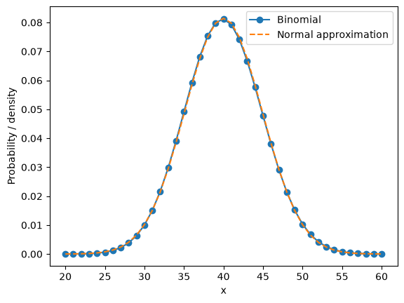

The binomial distribution is represented by probabilities at individual integer values, whereas the normal distribution is represented by a continuous density.

For large $n$ , the two curves become increasingly similar after the appropriate scaling.

A broader perspective¶

The distributions introduced in Lectures 4 and 5 form a useful basic gallery.

Discrete distributions¶

Bernoulli: one success/failure experiment.
Binomial: number of successes in a fixed number of independent Bernoulli trials.
Geometric: number of trials until the first success.
Poisson: number of events in a fixed interval under a rare-event model.

Continuous distributions¶

Uniform: all values in a finite interval are equally likely in the sense of having constant density.
Exponential: waiting time between events in a memoryless model.
Normal: a central continuous model arising naturally in measurement and aggregation problems.

The distributions are not isolated formulas. They arise from different mechanisms:

\text{Bernoulli trials} \quad\longrightarrow\quad \begin{cases} \text{Binomial: count successes},\\ \text{Geometric: wait for first success}. \end{cases}

For rare events,

\text{Binomial} \quad\longrightarrow\quad \text{Poisson}.

For a large number of independent trials,

\text{Binomial} \quad\longrightarrow\quad \text{Normal approximation}.

The last transition is the beginning of a much more general phenomenon that will eventually lead to the central limit theorem.

Summary¶

In this lecture we introduced several fundamental continuous probability distributions.

For a continuous random variable $\xi$ with density $p_\xi$ ,

\mathbb{P}(\{a<\xi\leq b\}) = \int_a^b p_\xi(x)\,dx.

We studied:

Uniform distribution
$\xi\sim U(a,b).$
Exponential distribution
$\xi\sim\operatorname{Exp}(\lambda),$
including its memoryless property.
Normal distribution
$\xi\sim N(a,\sigma^2),$
with density
$p_\xi(x) = \frac{1}{\sqrt{2\pi}\sigma} \exp\left( -\frac{(x-a)^2}{2\sigma^2} \right).$

We also introduced the standardization

z=\frac{x-a}{\sigma},

which reduces normal probabilities to probabilities involving the standard normal CDF $\Phi$ .

Finally, we saw that the binomial distribution can be approximated by a normal distribution for large numbers of trials. The De Moivre-Laplace theorem provides the first example of this phenomenon.

In the next lecture we will move from the description of distributions to the numerical quantities associated with random variables, beginning with expectation, moments, variance, and standard deviation.